Modelling the economic trade-offs of irrigation pipeline investments for improved energy management

 

 

Marcill Venter^*; Bennie Grové

PO Box 339, Department of Agricultural Economics, University of the Free State, Bloemfontein, 9300, South Africa

 

 

---

ABSTRACT

Higher electricity tariffs have accentuated the importance of the trade-off between lowering investment cost by buying pipes with smaller diameters and the higher operating costs that result from the increased power requirement to overcome the higher friction losses of the thinner pipes. The Soil Water Irrigation Planning and Energy Management (SWIP-E) mathematical programming model was developed and applied in this paper to provide decision support regarding the optimal mainline pipe diameter, irrigation system delivery capacity and size of the irrigation system. SWIP-E unifies the interrelated linkages between mainline pipe diameter choice and the timing of irrigation events in conjunction with time-of-use electricity tariffs. The results showed that the large centre pivot resulted in higher net present values than the smaller centre pivot and the lower delivery capacities were more profitable than higher delivery capacities. More intense management is, however, necessary for delivery capacities lower than 12 mm-d-1 to minimise irrigation during peak timeslots. Variable electricity costs are highly dependent on the interaction between kilowatt requirement and irrigation hours. For the large centre pivot the interaction is dominated by changes in kilowatt whereas the effect of irrigation hours in relation to kilowatts is more important for smaller pivots. Optimised friction loss expressed as a percentage of the length of the pipeline was below 0.6%, which is much lower than the design norm of 1.5% that is endorsed by the South African Irrigation Institute. The main conclusion is that care should be taken when applying the friction loss norm when sizing irrigation mainlines because the norm will result in pipe diameters that are too small, consequently resulting in increased lifecycle operating costs. A clear need for the revision of the friction loss design norm was identified by this research.

Keywords: Non-linear programming, economic trade-off, electricity costs, irrigation system investment costs, water management, net present value

---

 

 

INTRODUCTION

During the 1990s Eskom followed a pricing strategy whereby they wanted to supply South Africa with the lowest electricity costs in the world (Eskom, 2000). For many years electricity tariffs increased below the inflation rate resulting in a real decrease in electricity tariffs. In the early 2000s Eskom changed their pricing strategy and electricity tariffs have been increasing at rates above inflation since 2003. More alarming are the tariff hikes that have occurred since 2008 to finance new power plants to ensure that enough energy is supplied to satisfy an ever-increasing demand for energy in South Africa.

The impact of higher electricity costs is compounded by the fact that the irrigation systems that were designed when electricity costs were low are not energy efficient because more emphasis was placed on lowering investment costs compared to lowering energy costs. A trade-off exists between lowering investment cost by means of buying pipes with smaller diameters and the higher operating costs resulting from an increase in the power requirement to overcome the higher friction losses of the thinner pipes. As a result many farmers may be paying excessively high electricity costs due to irrigation system designs that are not energy efficient.

Various research techniques, such as Laybe's method, Lagrange multipliers, linear programming, dynamic programming, non-linear programming and recursive programming have been applied by numerous researchers (e.g. Laybe, 1981; Radley, 2000; Theocharis et aL, 2010; Planells et al., 2007; Pedras et al., 2009; Gonzalez-Cebollanda and Macarulla, 2012; Dercas and Valianthas, 2012) to evaluate the economic trade-off between investment costs and electricity costs. Although sound results were obtained from the methods the following critical assumptions were made:

• The irrigation system network layout must be known.

• A flat energy rate is used to calculate energy costs of an irrigation system.

• The annual operating time of an irrigation system is assumed.

Under a flat-rate electricity tariff structure the timing of irrigation events is unimportant because the irrigator is unable to manage electricity cost through adjustments to the timing of irrigation events which justifies an assumed annual operating time. Timing of irrigation events is of the utmost importance when considering time-of-use electricity tariffs because the irrigator is able to manage electricity costs by changing the timing of irrigation events.

Evaluating the economic trade-off between pipeline investment costs and operating costs when using time-of-use electricity tariffs is, therefore, complicated and requires the integration of irrigation system design components and irrigation scheduling in conjunction with time-of-use electricity tariffs. Such a holistic approach to energy management is supported by Jumman (2009). The problem is that currently no integrated modelling framework that satisfactorily integrates irrigation system design, irrigation water management and the use of alternative electricity tariff structures exists to provide decision support to South African farmers. As a result the Water Research Commission (WRC) of South Africa solicited research with respect to 'the optimisation of electricity and water use for sustainable management of irrigation farming systems' (WRC Project K5/2279) in order to improve the profitability of farming systems under increasing energy costs (WRC, 2014).

As part of the WRC project an integrated non-linear programming model that unifies the interrelated linkages between mainline pipe diameter choice and the timing of irrigation events in conjunction with electricity tariff choice was developed to facilitate better evaluation of the economic trade-offs of irrigation pipe investments for improved energy management. The main objective of this paper is to provide a description of the programming model and to demonstrate how it could be applied to provide decision support regarding pipeline investments.

SWIP-E programming model

The following section describes the Soil Water Irrigation Planning and Energy management programming model (SWIP-E) that is used to model the trade-off between pipeline investments and energy operating costs. The SWIP-E programming model is based on the SAPWAT optimisation (SAPWAT-OPT) (Grové, 2008) model that optimises a daily soil water budget for a single crop. The SAPWAT-OPT model was further developed in this research to facilitate inter-seasonal crop water use optimisation. Detailed electricity cost calculations and a mainline pipe optimisation model (Radley, 2000) were also included in the model to facilitate electricity energy management in an integrated way.

Objective function

The objective function maximises the net present value (NPV) of an irrigation system investment while considering the operating cost of the system. Specifically, the NPV is calculated as follows:

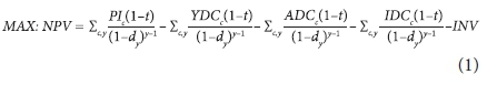
where: PI_c is the total production income (R = South African Rands) for crop c; YDC is the total yield-dependent costs (R) for crop c; ADC is the total area-dependent costs (R) for crop c; IDC is the total irrigation-dependent costs (R) for crop c; INVis the after-tax investment costs (R) for an irrigation system; t is th marginal tax rate (%) and d_yis the real discount rate (fraction) in year y.

The first 4 terms of the objective function calculate the NPV of the margin above specified costs for a specified crop rotation. The margin above specified costs (cash flow) is calculated by subtracting the yield, area and irrigation-dependent costs from the production income. The cash flow, with an exception of electricity costs, is calculated using constant prices; thus, real prices are used. Electricity costs are increased using a real increase in electricity tariffs (increase rate above inflation). The real discoun rate is calculated using the methodology proposed in Boelhje end Eidman (1984). The NPV is calculated by subtracting the after-tax investment costs of an irrigation system from the margin above specified costs.

Production income

Production income is a function of yield and area planted for each crop and the price of the crop. The production income for each crop considered in the model is calculated with the following equation:

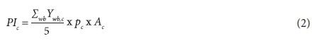
where: Y_wbc is the yield (t-ha^-1) for water budget wb for crop c; p_c is the crop price (R-t^-1) for crop c; A_c is the area (ha) planted to crop c.

Production income is calculated by multiplying the crop yield with the crop price and area planted. The crop price is an input in the model while the crop yield and area planted are endogenously determined in the model. The impact of nonuniform water applications is modelled through the inclusion of 5 water budgets, each receiving a different amount of water. The sum of the yields obtained in each water budget is divided by the number of water budgets to calculate the average crop yield that is used to calculate production income.

Yield-dependent costs

The calculation of yield-dependent costs is based on a cost-reduction method (Grové and Oosthuizen, 2002) and is calculated with the following equation:

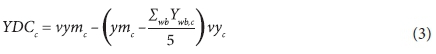
where: vym_c is the total yield-dependent costs (R) for crop c at maximum yield potential; ym is the maximum yield potential (t-ha^-1) for crop c; vy_c is a scaling factor for a less than proportional reduction in yield-dependent costs (R-t^-1) for crop c.

The first part of the equation represents total yield-dependent costs at maximum crop yield. The second part of the equation calculates the less than proportional reduction in yield-dependent costs for the difference between the maximum and actual yield by multiplying the difference with a scaling factor (vy_c). The following example is used to explain the calculation of the scaling factor. Suppose the yield-dependent costs to produce 17 t-ha^-1 and 13 t-ha^-1 of maize are R13 507 and R9 123/ha, respectively. The scaling factor is then calculated by dividing the cost reduction (R4 384/ha) by the yield reduction (4 t-ha^-1) to produce the scaling factor (R1 096/t) signifying the yield-dependent cost reduction per ton of reduced yield.

Area-dependent costs

Area-dependent costs include all input costs which will change with a change in the area planted. The area-dependent costs are calculated for each crop considered in the model by:

where: A_c is the area (ha) planted to crop c; va_cis the area-dependent cost (R-ha^-1) for crop c.

Irrigation-dependent costs

Irrigation-dependent costs are a function of the pumping hours necessary to apply irrigation water, and are calculated with the following equation:

where: EC_cis the total electricity cost (R) for crop c; LC_cis the total labour cost (R) for crop c; RMC_cis the total repair and maintenance cost (R) for crop c, and WC_c is the total water cost (R) for crop c.

Irrigation-dependent costs (IDC) include electricity costs, labour costs, repair and maintenance costs, and the water tariff paid. Total electricity costs depend on the type of electricity tariff. All tariff options include a fixed (paid every month irrespective of whether electricity was used) cost and variable (paid for the electricity consumed) cost. Variable electricity costs are a function of management (hours pumped), electricity tariffs and irrigation system design (kW). Electricity costs are calculated with the following equation:

where: PH_i,t. is pumping hours on day i in timeslot t; kW is the kilowatt (kW) requirement; kvar is the kilovar (kVAR); ta_it is the active energy charge (R-kWh^-1) on day i in timeslot t; tra_it is the reactive energy charge (R-kVARh^-1) on day i in timeslot t; rc_it is the reliable energy charge (R-kWh^-1) on day i in timeslot t; dc is the demand energy charge (R-kWh^-1) on day i in timeslot t, and fec is the fixed electricity cost (R).

The electricity tariffs are divided into different charges, i.e., active, reliable and demand energy charge, which is dependent on the product of the kW requirement of an irrigation system and the pumping hours. The kW requirement is closely linked to irrigation system layout and design. Pumping hours (PH) is determined by irrigation management and the limits that are placed on irrigation hours during the irrigation cycle when using time-of-use electricity tariffs. The reactive energy charge is dependent on the kilovar (kVAR) and pumping hours of an irrigation system. The kvar is calculated from the power factor (PF) of the pump (kVAR = cos^-1 PF). Each pump has a unique power factor which can be obtained from the manufacturer. The user pays for 70% of the kvarh used. The fixed electricity costs (fec) are an input parameter in the model and depend on the type of electricity tariff.

Equations 7 and 8 represent the formulas to calculate labour costs and repair and maintenance costs of the irrigation system, respectively. The calculation procedures for labour and repair and maintenance costs are based on formulas proposed by Meiring (1989). Specifically, labour costs are calculated as follows:

where: lh is the labour hours needed per 24 h irrigation for a given size centre pivot and is the labour wage (R/h).

Labour costs for permanent labourers can be considered as a fixed cost. However, labour costs obtain a variable character once labour is employed in a specific enterprise because labour costs can then be allocated between different enterprises. Labour costs for centre pivot irrigation are variable because the labour hours required are determined by the hours that the system is operational. The amount of labour that is required per operating hour is influenced by the size of the system and the type of task being performed. The model calculates the labour demand for every 24 h that the system is operated. The calculated labour demand is multiplied with the total pumping hours and the labour wage to calculate total labour costs.

Repair and maintenance costs depend on the conditions (climate) under which the system operates. The pump's repair and maintenance cost is directly linked to the use of the pump, through expressing the repair and maintenance tariff as a percentage per 1 000 hours pumped. The repair and maintenance costs of the motor, pivot and pipe are not included in the model since these are independent of the use of the system and will decrease the profit linearly (Meiring, 1989). Repair and maintenance is calculated with the following equation:

where: rt is the repair and maintenance tariff per 1 000 h (R-1 000 h^-1) pumped for an irrigation system.

The following formula is used to calculate the water charge:

where: IR is the irrigation amount (mm) for crop c on day i and wt is the water tariff (R-mm^-1).

Water charge is a function of the total amount of irrigation water applied over the crop area and the water tariff charged by the water user association. The water tariff includes the totality of payments that an irrigator makes for the irrigation service and is calculated on a volumetric basis. The volumetric-based charge is a fixed rate per unit water received, where the charge is proportional to the volume of water received. The charge per millimetre water was calculated by dividing the total charge by the volume of water allocated.

Investment costs

The section describes the calculation procedures used to calculate the net after-tax investment costs of an irrigation system. The calculation procedure of the main pipeline is based on the formulas used in the linear programming pipe optimisation model developed by Radley (2000). The pivot and pump investment costs are obtained from a manufacturer and are inputs in the model. The following equation represents the calculation procedure for investment costs of an irrigation system:

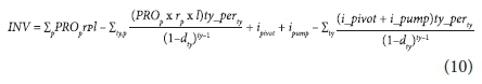
where: PRO_pis the proportion (fraction) of pipe p used; r_p is the cost (R-m^-1) of pipe p; l is the length (m) of the main pipeline; ty_per_tyis the tax deduction (%) in tax year ty; d_tyis the real discount rate (fraction) in tax year ty; i_pivot is the investment cost (R) of the pivot; i_pump is the investment cost (R) of the pump and tb is the tax benefit (R) received in tax year ty for a pivot and pump investment.

The main pipeline can be designed by choosing the pipe diameter such that the sum of the operating and investment costs is minimised. Calculations are done with consideration of the investment of the pipe, the tax benefit that the irrigator will receive from investing in a new pipeline and electricity costs (operating costs). Investment costs depend on the pipe costs and length of the pipe, and can be considered as a lump sum. The cost of the pipes and the length of the main pipeline are inputs in the model. The tax benefit that the irrigator will receive from investing in a new irrigation system was included in the calculation of the investment costs of the main pipeline, centre pivot and pump. The tax benefit calculations are based on a 50%, 30% and 20% tax deduction, respectively, in Year 1, 2 and 3. The present value of the tax benefit was calculated by using the same procedure as in the objective function.

Equation 11 is included in the model to ensure that sum of the proportions of the pipes used equals 1:

Constraint set

The following section describes the constraint set of the SWIP-E model. The section is divided into crop yield calculations, pumping hours, kilowatt requirement calculation, and resource constraints.

Crop yield and water budget calculations

Crop yield is calculated with the use of crop yield response factors (ky) which relate relative yield decrease (1-Y/Ym) to relative evapotranspiration deficit (1-ETA/ETM). The Stewart multiplicative relative evapotranspiration formula (De Jager, 1994) was used to calculate crop yield taking the effect of water deficits in different crop growth stages into account. Specifically, crop yields were calculated with the following equation:

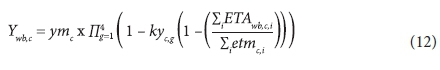
where: ky_cg are the yield response factors for crop c in growth stage g, ETA_wbCiJis the actual evapotranspiration in water budget wb for crop c on day i (mm) and etm_ci is the maximum evapotranspiration for crop c on day i (mm).

The only variable influencing crop yield in Eq. 12 is the level of actual evapotranspiration (ETA) which is calculated with the following equation:

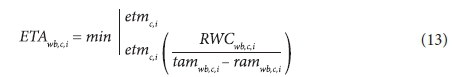
where: RWC_wb,c,i, . is the root water content in water budget wb for crop c on day i (mm), tam_wbci is the total available moisture in water budget wb for crop c on day i (mm) and ram_wb is the readily available moisture in water budget wb for crop c on day i (mm).

Equation 13 shows that ETA is determined by the root water content of the soil which dynamically changes over the growth season of the crop as it is influenced by crop water demand and irrigation events. Thus, water budget calculations are necessary to determine actual evapotranspiration. The water budget routine included in the SWIP-E model originates from the SAPWAT model (Crosby and Crosby, 1999) and distinguishes between water in the root zone and below the root zone. The total available moisture in the soil that potentially can be used by the crop is a function of the water-holding capacity of the soil and the rooting depth of the crop. Only a portion of tam is readily available for crop consumption. ram is a function of root development, water-holding capacity of the soil and the P-value, which indicates the proportion of the water that is readily available for crop consumption. The P-value calculation is based on a formula proposed in Dominguez et al. (2012). If soil moisture deficits are greater than ram, the rate at which the crop consumes water is reduced from its potential level and ETA is only a fraction of etm.

Irrigation systems do not apply water with perfect uniformity. Due to the lack of uniformity a part of the field is adequately irrigated while others are not. Various researchers (Hamilton et al., 1999; Grové and Oosthuizen, 2010; Lecler, 2004) modelled the impact of non-uniformity by dividing the irrigation field into different water budgets. The relationship between applied water and crop yield was explicitly incorporated in the water budget calculations by modelling 5 different water budgets simultaneously in SWIP-E. Crop yields were estimated for each of the water budgets included in the model to take cognisance of nonuniform water applications.

Modelling a daily water budget within a mathematical programming framework is complex and the reader is referred to Venter (2015) for a detailed description of the necessary equations to model a two-layer daily soil water budget.

Pumping hours

The pumping hours required to apply a certain amount of water are calculated according to Burger et al. (2003) with the following equation:

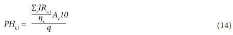
where: q is the flow rate (m³-h^-1) and η is the irrigation system application efficiency (%).

The irrigation amount is calculated in the model, while the flow rate and irrigation system application efficiency are input parameters in the model. The irrigation amount is based on the average irrigation of the water budgets included in SWIP-E to model non-uniform water applications. The irrigation system application efficiency is used to account for spray losses (wind drift).

Eskom's time-of-use electricity tariffs are designed to create an incentive for irrigation farmers to use electricity during low-demand season and off-peak hours. The time-of-use tariffs are divided in 3 time-slots with different rates applicable to each time-slot. Pumping hours are restricted to the available hours within an irrigation cycle and time-of-use time-slot with the following equation:

where: thc are the available irrigation hours within each irrigation cycle on day i in time-slot t (h).

The basic idea is that pumping hours in a specific time-slot cannot exceed the available irrigation hours in that specific time-slot.

Kilowatt requirement

Kilowatt (kW) is determined endogenously in the model and quantifies the kilowatts required to drive the water through the system. Kilowatt is a function of the flow rate of the pump, total pressure required by the system and the efficiency of the pump and motor (Burger et al., 2003). Equation 16 is used to calculate the kilowatt requirement at the pumping station:

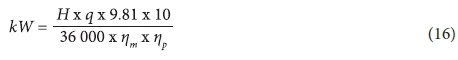
where: H represents the total pressure required by the system (m), n_m is the motor efficiency (%) and n_p is the pump efficiency (%).

Total pressure in the system is the sum of the operating pressure of the pivot, static head and friction in the main pipeline. The pivot pressure represents the required pressure at the centre of the pivot in order to apply a designed irrigation amount per day. Static head is a constant which represents the difference in elevation between the water source and the irrigation system. Equation 17 is used to determine the total operating pressure of the system which the pump must supply:

where: hs is the static head (m) and f_pis the friction loss associated with each pipe diameter for a given flow rate (m).

Friction in the mainline is a function of the proportion of the pipe diameter that has been used in the mainline and the friction that was calculated through the use of the Darcy-Weisbach (Burger et al., 2003) equation for a given flow rate.

Area

The following equation is used to restrict the area planted of a certain crop to the pivot size:

The model is developed for a crop rotation system consisting of maize and wheat. Thus, the available area for each crop must be equal to or smaller than the designed centre pivot size. Important to note is that the model does not model intra-sea-sonal competing crops since the crop rotation consists of maize and wheat only.

Water

The maximum amount of water that could be applied within a year is determined by the water user association. Equation 19 is used to restrict the amount of irrigation water applied (average water budget) not to exceed the water quota:

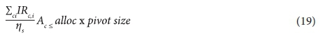
where: alloc is the water quota (m³-ha^-1).

Equation 20 restricts individual irrigation events to a user-specified maximum irrigation application within an irrigation cycle. The user has to specify the length of an irrigation cycle which determines the timing of an irrigation event. The constraint is used to ensure that the infiltration rate of the soil is not exceeded.

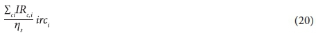
where: irc. is the irrigation amount per cycle for crop c on irrigation day i (mm-cycle^-1).

The above resource constraints are explicitly included in the modelling process.

Model application and inputs

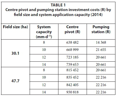
The model was applied in the Douglas area to optimise the mainline design for 2 irrigated field sizes (30.1 ha and 47.7 ha) most commonly found in the area. The irrigation systems are designed with one centre pivot on the main pipeline with a length of 750 m. Thus, only one operating point exists. A static head of 12 m was assumed for the analyses. Four different irrigation system application capacities ranging from 8 to 14 mm-d^-1 were included in the analyses to demonstrate the importance of irrigation system application capacities on the ability to exploit time-of-use electricity tariff structures to reduce irrigation costs.

Centre pressure, flow rate and efficiency of the pump are necessary to calculate kilowatt requirement in the model. The centre pressure, flow rate and the efficiency of the pump depend on the size and capacity of the centre pivot and will vary between different centre pivot designs.

Capital requirements

The amount of capital required to invest in an irrigation system is a function of field size, flow rate, system pressure and the distance from the water source. Irrigation system design data for the eight scenarios were obtained from a local SABI-accredited irrigation system designer (Myburgh, 2014).

Mainline costs are dependent on the pipe diameter, which is a variable in the model, whereas centre pivot and pumping station costs are an input in the model (Table 1). The investment costs were collected from personal communications with an irrigation designer (Myburgh, 2013).

 

 

Operating costs

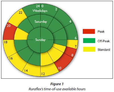
An important decision for irrigation farmers in South Africa is the decision to choose between Ruraflex and Landrate (electricity tariff options). Ruraflex consists of a time-of-use option where Landrate is a flat rate. Both of the electricity tariffs consist of variable and fixed charges. The variable energy charges for Landrate include energy (c-kWh^-1), reliability service (c/kWh) and network demand charge (c-kWh^-1), while the fixed tariffs, which depend on the point of delivery (POD), include a service (R/POD per day) and a network access charge (R/POD per day). All of the tariffs applicable to Landrate depend on the Landrate option (Landrate 1, 2, 3, 4 or Dx) the irrigator uses. The variable energy charges for Ruraflex include active energy (c/kWh), reliability service (c-kWh^-1), network demand (c/kWh) and reactive energy charge (c-kVARh^-1), while the fixed tariff consists of network access (R-KVA^-1-m^-1), service (R-account^-1-d^-1) and administration charges (R-POD^-1-d^-1). The reliability service and network demand charge is dependent on the voltage size, while the service and administration charge is dependent on the monthly utilised capacity. The reactive energy charge is differentiated by the demand season. The active energy charge applicable to Ruraflex depends on the transmission zone (distance from the power station) and voltage size, and is differentiated by demand seasons (high and low) and time-of-use periods. Figure 1 illustrates the time-of-use hours available in each time-slot. The available hours are different between weekdays and weekends. During the week there are 8 off-peak hours, 11 standard hours and 5 peak hours available. The weekends consist of only standard and off-peak hours (Eskom, 2014/15).

 

 

A minimum wage of 12.41 R-ha"¹ is used in the application of the model (DOL, 2014). The labour requirement for every 24 h that the irrigation system operates is based on the data proposed in Meiring (1989) and amounts to 0.58 labour h per 24 h. The repair and maintenance tariff calculated depends on the irrigation system design and is based on a method proposed by Meiring (1989). The tariff is a function of the initial investment of the pump and is expressed as a cost per 1 000 hours pumped. The water tariff depends on the water user association which is based on a volumetric-based charge with an allocation of 10 000 m³-ha^-1. The tariff per millimetre water applied is calculated by dividing the tariff with the water allocation and is equal to 0.716 R-mm^-1.

Irrigation system design

Friction in the main pipeline is included as a parameter in the model. Equation 21 was used to calculate friction in the main pipeline through the use of the Darcy-Weisbach equation (Burger et al., 2003) in combination with the Hazen-Williams (Burger et al., 2003) equation and is given by:

where: f_pis the friction loss (m) for pipe p; k is the pipe roughness (mm); d is the inside pipe diameter (mm) and Re is the Reynolds number.

Water budget parameters

All relevant input parameters that are necessary in the calculation of the water for maize and wheat are included in this section. Maize is a short grower with a growing period of 120 days while a spring type wheat cultivar is used with a growing period of 148 days. Weather data for 49 years were obtained from Van Heerden (2012). The weather station is situated in a dry and hot climate area. The weather data include rainfall and potential evapotranspiration (ET0) on a daily basis for maize and wheat. Potential evapotranspiration (ET0) together with the Kc values are used to calculate maximum evapotranspiration. Equation 22 is used to calculate maximum evapotranspiration (ETM) for each crop considered in the model:

In addition to weather data inputs regarding the soil, root development, yield response factors and water allocation are also required. A low water-holding capacity (WHC) of 100 mm-m"¹ and a soil with a depth of 1.2 m was used in the analysis. The initial depletion of both of the soils was taken as 50% depletion to calculate the RWC and BRWC on the first day of the water budget. Only a portion of TAM is readily available for crop consumption; therefore, the P-value (Dominguez et al., 2012) of maize and wheat was calculated on a daily basis.

The root development of maize and wheat was collected from Van Heerden (2012). The root growth for maize and wheat was 0.3 m for the initial stage and developed from 0.3 m to 1.2 m between the crop development and mid-season stage, which is the maximum root growth for maize and wheat. As the roots of the crop develop the ground cover, crop height and the leaf area change. The growing period can be divided into 4 distinct growth stages, namely, initial, crop development, mid-season, and late season.

Yield response factors are crop specific and vary over the growing season according to the growth stages. If Ky > 1 the crop response is very sensitive to water deficit with proportionally larger yield reductions when water is reduced because of stress. If Ky < 1 the crop is more tolerant to water deficits and recovers partially from stress resulting in less than proportional reductions in yield with reduced water use. If Ky = 1 the yield reduction is directly proportional to reduced water use. The yield response factors (Ky coefficients) and the length of the stages (Ky days) are based on values proposed in Doorenbos and Kassam (1979). Potential yield for maize and wheat cultivated under irrigation is assumed as 17 t-ha^-1 and 8 t-ha^-1, respectively.

Non-uniformity of irrigation applications are modelled through the inclusion of 5 water budgets. Two water budgets received more than the average while two received less than the average amount of water. The applied irrigation for each of the five water budgets was calculated by multiplying the average applied water with a scaling factor (cu scale).

The water allocation was taken as 1 000 mm-ha^-1 (10 000 m³-ha^-1). The assumption is made that the calculated irrigation amount will not exceed 15 mm-cycle^-1 within an irrigation cycle of 2 days, due to the infiltration ratio of the soils and the application ratio of the pivot at the end.

 

RESULTS

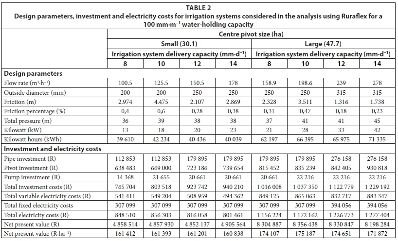
The results obtained from the economic evaluation for pipe investments are presented in this section. The section includes the results obtained for Ruraflex. Table 2 shows the design parameters, investment and electricity costs as well as the profitability of Ruraflex for the eight different irrigation systems included in the analysis for a low water-holding capacity of 100 mm-m^-1. The irrigation systems include a small (30.1 ha) and large (47.7 ha) centre pivot with irrigation system delivery capacities ranging from 8 mm-d^-1 to 14 mm-d^-1. If irrigation system delivery capacities increase from 8mm/d to 14 mm-d^-1 the flow rates increase from 100.5 m³-h^-1 to 178 m³-h^-1 for the small centre pivot and from 158.9 m³-h^-1 to 278 m³-h^-1 for the large centre pivot. Low system delivery capacities (8 mm-d^-1 and 10 mm-d^-1) resulted in thinner optimal pipe diameters when compared to higher system delivery capacities (12 mm-d^-1 and 14 mm-d^-1). For example, the most economical pipe diameter for the low system delivery capacities for the small centre pivot is 200 mm while a 250 mm pipe diameter is optimal for the higher system delivery capacities. Larger pipe diameters are optimal for the large centre pivot compared to the small centre pivot when comparing systems with the same delivery capacities. The optimal pipe diameters increase by 50 mm and 65 mm, respectively, for low and high system delivery capacities when increasing centre pivot size. These changes in pipe diameters are a direct result of the higher flow rates associated with larger pivots.

Changes in pipe diameter and flow rate (delivery capacity) have a direct impact on the kilowatt requirement to drive the water through the system and, therefore, operating costs. If the pipe diameter stays the same friction increases as the flow rates increase, resulting in an increase in the kilowatt requirement. Friction increases from 2.974 m to 4.475 m if the flow rate increases from 100.5 m³-h^-1 to 125.5 m³-h^-1, resulting in a 5 kW increase in the kilowatt requirement. The optimal pipe diameter increased when flow rate increased from 125.5 m³-h^-1 to 150.5 m³-h^-1 which resulted in a decrease in friction even though the flow rates increase. Larger pipe diameters reduce friction loss and, therefore, total pressure with lower kilowatt requirements, while increases in flow rate will cause an increase in kilowatt requirement. The direction of change in kilowatt requirement is, therefore, not self-evident if pipe diameter is increased in conjunction with an increase in flow rate. The results show that the kilowatt requirement will increase, but that this is less than proportional. For example, if the flow rate is increased from 125.5 m³-h^-1 to 150.5 m³-h^-1 for the small centre pivot the friction decreases from 4.475 m to 2.107 m resulting in an increase in kilowatt requirement of 2 kW. The same observation is made for the large centre pivot. The percentage friction followed the same trend as the friction loss since the length of the main pipeline is constant. Important to note is that the percentage friction loss is much less than the norm of 1.5%. The results show that friction loss as a percentage of the length of the pipe never exceeds 0.6%. The implication of using the 1.5% norm is that thinner pipe diameters would be used which decrease investment cost but at the same time increase operating cost (electricity cost). Thus, increasing electricity costs will have a significant effect on the profitability of irrigation systems if thinner pipes are used.

The results show that variable electricity costs increase as flow rate increases if the optimal pipe diameter stays the same. However, variable electricity costs decrease if the optimal pipe diameter increases in conjunction with flow rate increases. For example, if the flow rate increases from 158.9 m³-h^-1 to 198.6 m³-h^-1, variable electricity costs increase from R849 125 to R865 063 when pipe diameter is constant and decrease from R865 063 to R832 717 if the flow rate increases to 239 m³-h^-1 and the optimal pipe diameter increases Generalisations are, however, not possible since variable electricity costs decreased between the 12 mm-d^-1 and 14 mm-d^-1 irrigation system delivery capacities for the small centre pivot even though pipe diameter stayed the same. The reason for the decrease in variable electricity costs is that the increase in kilowatt requirement is less than the decrease in irrigation pumping hours associated with irrigating with higher system delivery capacities, which resulted in a decrease in kilowatt hours (kWh). The kilowatt hours decreased with 397kWh (40 436kWh - 40 039kWh) which caused a decrease in variable electricity costs of R14 597 (R508 959 - R494 362) between the 12 mm-d^-1 and 14 mm-d^-1 irrigation system delivery capacities for the small centre pivot. The interaction between kilowatt requirement and the pumping hours emphasises the importance of appropriately modelling the interaction between irrigation system design and management. Fixed electricity costs are the same (R307 099) for all the irrigation systems except for the high irrigation system delivery capacities (12 mm-d^-1 and 14 mm-d^-1) for the large centre pivot due to a higher kilovolt-ampere point. The fixed electricity costs for the high system delivery capacity for the large centre pivot is R394 056 due to a 75 KVA point. Total electricity costs for the large centre pivot increase as flow rate increases due to the increase in fixed electricity costs.

Net present value (NPV) decreases as flow rate increases for the small centre pivot with an exception for an increase between the 12 mm-d^-1 and 14 mm-d^-1 delivery capacities. The increase is due to a slightly larger irrigated area (ha) which causes total NPV to increase. However, NPV per hectare decreases as flow rate increases for the small centre pivot. Increasing investment costs resulted in a decrease in NPV per hectare. The 8 mm/d delivery capacity resulted in the most profitable irrigation system delivery capacity for the small centre pivot. The NPV of the large centre pivot increases between the 8 mm-d^-1 and 10 mm-d^-1 irrigation system delivery capacities and decreases for delivery capacities above 10 mm-d^-1. The 10 mm-d^-1 delivery capacity resulted in the highest NPV for the large centre pivot. Even though electricity costs and investment costs increased between the 8 mm-d^-1 and 10 mm-d^-1 delivery capacity, the NPV is highest for the 10 mm-d^-1 delivery capacity because the crop yield for wheat was slightly higher resulting in higher gross margins. Again the increase in total investment costs is responsible for the decreasing trend in NPVs for irrigation system delivery capacities above 10 mm-d^-1 for the large centre pivot.

Table 3 shows the optimised pumping hours for the alternative irrigation system designs using the Ruraflex electricity tariff. Total optimal pumping hours decrease as flow rate increases between irrigation system delivery capacities for both the centre pivot sizes. Higher flow rates can apply more water in 1 h, thus, fewer irrigation hours are necessary to apply the same amount of irrigation water.

Small variations in total irrigation hours are present between the centre pivot sizes for a given irrigation system delivery capacity. Total irrigation hours for the 8 mm-d^-1 delivery capacity is 2 995 h for the small centre pivot and 3 002 h for the large centre pivot. However, the distribution of irrigation hours between maize and wheat are different. The shift in irrigation hours towards maize is to reduce pumping of water during the portion of wheat's growing season that falls in the high energy demand season when the Ruraflex electricity tariff is very high. The results further show that the pumping hours in each of the time-of-use time-slots are less than the available pumping hours in a specific time-slot. The last mentioned is because the timing and magnitude of water applications are dictated by the status of the crop which is related to the soil water availability. The distribution of pumping hours within each of the time-of-use time-slots shows that maize is mostly irrigated during off-peak and standard time, while wheat needs to be irrigated during peak times when considering irrigation system delivery capacities below 12 mm-d^-1. The value of the marginal product is much higher than the marginal factor cost of applying irrigation water; therefore, it is profitable to irrigate during peak time-slots. For irrigation system deliveries above 10 mm-d^-1 the capacities are such that enough water could generally be applied to minimise irrigation during peak time-slots.

 

CONCLUSION

SABI-accredited designers are allowed to design irrigation systems such that the friction as a percentage of the length of the pipeline does not exceed 1.5%. The implication of the norm is that smaller pipe diameters are installed which result in higher operating costs due to an increase in kilowatt requirement. From the results of this study the highest friction percentage for optimal pipe diameters was 0.6% and 0.47% for the small and large centre pivot, respectively. Thus, the conclusion is that the SABI design norm is much higher than the friction percentages of optimal pipe diameters and should be lowered to ensure that there is a better balance between investment and operating costs.

An important factor that determines total variable electricity costs is the product of kilowatt and pumping hours. Pumping hours are reduced if the irrigation system delivery capacity is increased. The degree of reduction is almost the same between the small and large centre pivots. However, significant differences exist between the small and large centre pivots in terms of increasing kilowatt requirements associated with increasing delivery capacities. Kilowatt requirements increase with 10 kW and 21 kW, respectively, for the small and large centre pivot. The magnitude of the increase in kilowatt requirement for the large pivot causes the kilowatt hours to increase even though pumping hours are reduced with increasing delivery capacities. The relatively small change in kilowatt requirements necessary to increase delivery capacity for the small pivot causes kilowatt hours not to increase significantly with increasing delivery capacity. The direction of change in the kilowatt hours for the small centre pivot depends more on the interaction between increasing kilowatt requirement and decreasing pumping hours resulting from increasing delivery capacities. Thus, the conclusion is that the interaction between kilowatt requirement and irrigation management (hours) becomes more significant for smaller irrigated areas in determining variable electricity costs.

Intense management is required for smaller irrigation system delivery capacities, because longer irrigation hours are needed in order to avoid a decrease in crop yield. The timing of irrigation is of utmost importance since it has a direct effect on electricity costs and crop yield. The assumption made by various researchers and irrigation designers that all available off-peak hours will be used first before irrigation will take place in more expensive time-of-use time-slots is voided by the fact that the water budget and the status of the crop will determine irrigation timing and amounts.

 

ACKNOWLEDGMENTS

The Water Research Commission (WRC) of South Africa is gratefully acknowledged for initiating, funding and managing the research project 'The optimisation of electricity and water use for sustainable management of irrigation farming systems' (WRC project K5/2279). The views of the authors do not necessarily reflect those of the WRC.

 

REFERENCES

BOEHLJE MD and EIDMAN VR (1984) Farm Management. John Wiley and Sons, New York.         [ Links ]

BURGER JH, HEYNS PJ, HOFFMAN E, KLEYNHANS EPJ, KOEGELENBERG FH, LATEGAN MT, MULDER, SMAL HS, STIMIE CM, UYS WJ, VAN DER MERWE FPJ, VAN DER STOEP I and VILJOEN PD (2003) Irrigation Design Manual. ARC-Institute for Agricultural Engineering, Pretoria.         [ Links ]

CROSBY CT and CROSBY CP (1999) SAPWAT: A computer program for establishing irrigation requirements and scheduling strategies in South Africa. WRC Report No. 624/1/99. Water Research Commission, Pretoria.         [ Links ]

DE JAGER JM (1994) Accuracy of vegetation evaporation ration formulae for estimating final wheat yield. Water SA 20 307-314.         [ Links ]

DERCAS N and VALIANTZAS JD (2012) Two explicit optimum design methods for a simple irrigation delivery system: Comparative application. Irrig. Drain.61 10-19. http://dx.doi.org/10.1002/ird.632        [ Links ]

DOMINGUEZ A, DE JUAN JA, TARJUELO JM, MARTINEZ RS and MARTINEZ-ROMERO A (2012) Determination of optimal regulated deficit irrigation strategies for maize in a semi-arid environ ment. Agric. Water Manage.110 67-77. http://dx.doi.org/10.1016Aj.agwat.2012.04.002        [ Links ]

DEPARTMENT OF LABOUR (2014) Minimum wage for farm worker sector with effect from 1 March 2014. Department of Labour, South Africa.         [ Links ]

DOORENBOS J and KASSAM AH (1979) Yield Response to Water. Food and Agriculture Organization of the United Nations.         [ Links ]

ESKOM (2000) Tariff and charges booklet. URL: http://www.Eskom.co.za/CustomerCare/TariffsAndCharges/Documents/2000a.pdf [(Accessed 21 January 2016).

ESKOM (2014/15) Tariffs and charges booklet. URL: http://www.Eskom.co.za/content/2014_15DraftTariffBookver3.pdf (Accessed 21 January 2016).         [ Links ]

GONZALEZ-CEBOLLADA C and MACARULLA B (2012) Comparative analysis of design methods of pressurized irrigation networks. Irrig. Drain. 61 1-9. http://dx.doi.org/10.1002/ird.657        [ Links ]

GROVÉ B (2008) Stochastic efficiency optimisation analysis of alternative agricultural water use strategies in Vaalharts over the long- and short-run. PhD thesis, University of the Free State, Bloemfontein.         [ Links ]

GROVÉ B and OOSTHUIZEN LK (2002) An economic analysis of alternative water use strategies at catchment level taking into account an instream flow requirement. J. Am. Water Resour. Assoc. 38 2. http://dx.doi.org/10.1111/j.1752-1688.2002.tb04324.x        [ Links ]

GROVÉ B and OOSTHUIZEN LK (2010) Stochastic efficiency analysis of deficit irrigation with standard risk aversion. Agric. Water Manage. 97 (6) 792-800. http://dx.doi.org/10.1016/j.agwat.2009.12.010        [ Links ]

HAMILTON JR, GREEN GP and HOLLAND D (1999) Modeling the reallocation of Snake River water for endangered salmon. Am. J. Agric. Econ. 81 1252-1256. http://dx.doi.org/10.2307/1244117        [ Links ]

JUMMAN A (2009) A framework to improve irrigation design and operating strategies in the South African sugarcane industry. MSc dissertation, University of KwaZulu-Natal.         [ Links ]

LABEY Y (1981) Iterative discontinuous method for networks with one or more flow regimes. In: Proceedings of the International Workshop on Systems Analysis of Problems in Irrigation - Drainage and Flood Control, 30 Nov-4 Dec 1981, New Delhi.         [ Links ]

LECLER N (2004) Methods, tools and institutional arrangements for water conservation and demand management in irrigated sugarcane. In: Proceedings of the 13^th International Soil Conservation Organisation Conference, July 2004, Brisbane.         [ Links ]

MEIRING JA (1989) 'n Ekonomiese evaluering van alternatiewe spil- puntbeleggingstrategieë in die Suid-Vrystaat substree met inagneming van risiko (Afrikaans). MSc dissertation, University of the Orange Free State.         [ Links ]

MYBURGH C (2014) Personal communication, July 2014. Cobus Myburgh, Valley, Douglas, South Africa, 8730.         [ Links ]

PEDRAS CMG PEREIRA LS and GONCALVES JM (2009) MIRRIG: a decision support system for design and evaluation of micro irrigation systems. Agric. Water Manage. 96 (4) 691-701. http://dx.doi.org/10.1016/j.agwat.2008.10.006        [ Links ]

PLANNELS P ORTEGA JF and TARJUELO JM (2007) Optimization of irrigation water distribution networks, layout included. Agric. Water Manage.88 110-118. http://dx.doi.org/10.1016/j.agwat.2006.10.004        [ Links ]

RADLEY R (2000) Sagteware vir die ontwerp van besproeiingstelsels - 'n ondersoek na geskikte pakkette (Afrikaans). ARC Institute for Agricultural Engineering, Pretoria.         [ Links ]

THEOCHARIS ME TZIMOPOULOS CD SAKELLARIOU- MAKRANTONAKI MA YANNOPOULOS SI and MELETIOU IK (2010) Comparative calculation of irrigation networks using Labye's method, the linear programming method and a simplified nonlinear method. Math. Comput. Model. 51 286-299. http://dx.doi.org/10.1016/j.mcm.2009.08.040        [ Links ]

VAN HEERDEN PS (2012) Personal communication, July 2014. Pieter van Heerden, PICWAT, Bloemfontein, South Africa, 9301.         [ Links ]

VENTER M (2015) Modelling the economic trade-offs of irrigation pipeline investments for improved energy management. MSc dissertation, University of the Free State.         [ Links ]

WRC (Water Research Commission) (2014) WRC Knowledge Review 2013/14. Water Research Commission, Pretoria.         [ Links ]

 

 

Received 15 January 2016
Accepted in revised form 6 September 2016

 

 

* To whom all correspondence should be addressed.+27 (0) 401 3450; e-mail: venterm5@ufs.ac.za