Numerical study of junction-angle effects on flow pattern in a river confluence located in a river bend

 

 

Rasool Ghobadian^{I, *}; Zahra Seydi Tabar^I; Parisa Koochak^II

^IDepartment of Water Engineering, PO Box 1158, Razi University, Kermanshah, Iran
^IIShahid Chamran University, PO Box 61357-43311, Ahvaz, Iran

 

 

---

ABSTRACT

The effect of main channel curvature on the flow pattern in river junctions is a complex and important issue. The 3-dimensional flow pattern in a river bend with a lateral or tributary channel is not only affected by the centrifugal force and pressure gradient but is also affected by the tributary channel's momentum. Understanding this phenomenon requires extensive research: in this study the effect of 4 tributary junction angles, placed at a 45° angle from the beginning of the bend, is studied using SSIIM1 software. The effect of the junction angle on the vertical and transverse velocity profile, water level changes in the main channel, bed shear-stress distribution and secondary flow strength were evaluated. The results showed that by increasing the junction angle from 30° to 115° the streamwise velocity in the vicinity of the centre line and the inner wall of the bend increases. Increasing the junction angle also increases the separation zone dimensions, maximum bed shear stress, difference between the upstream and downstream water level in the junction and the secondary flow strength.

Keywords: flow pattern, junction angle, 180 degree bend, SSIIM1 numerical model

---

 

 

INTRODUCTION

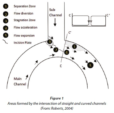
Water flow in rivers, especially meandering rivers, is very complex. This complexity is not only because of their turbulence and intense 3-dimensional nature but also because of their topography and depth variations. River junctions in natural meanders also increase the flow pattern's complexity. Although the effect of bending curvature on flow dynamics and sediment in channels has received a considerable amount of attention, only limited information about the effect of bending curvature on flow patterns in river junctions is available, and there have been very few studies considering river junctions in river bends. Roberts (2004) did an experimental and numerical investigation on river meanders. According to Roberts' study, the identified areas in straight and curved junctions are shown in Fig. 1.

 

 

The use of numerical models for simulating the flow in river junctions has recently attracted researchers' attention, such as Weerakoon et al. (1991), Huang et al. (2002), Biron et al. (2004) and Chen and Peng (2006). Weerakoon et al. (1991) used a fully elliptic treatment in study of a 60° asymmetrical confluence. They found that the predicted recirculation zone length in the downstream direction was approximately 30% too short. This was attributed to numerical diffusion associated with grid discretization, the use of a basic form of k-εtype turbulent model and the treatment of the water surface as a grid lid without appropriate correction of the mass conservation equation. Huang et al. (2002) presented a 3-dimensional model for a 90° junction with the ability to predict the changes in water level and used Weber's experimental data to calibrate his model. He first compared the simulation results for q*= 0.25 and q*= 0.75 with Weber's experimental data; then he examined the effect of the junction angle on the flow characteristics. Biron et al. (2004) used a 3-dimensional model to examine mixing processes immediately downstream of confluence as well as further downstream in the mainstream. Simulations are presented for concordant and discordant laboratory junction and a field confluence for a low and a high flow condition. The results showed that the decrease in standard deviation at a cross section of a tracer over a distance of 5 channel widths is 30% for discordant beds but only 10% for concordant beds in the laboratory simulation. Chen and Peng (2006) presented a 2-dimensional numerical model for a 2-layer flow, where each layer has a different velocity and density. They showed that the model can describe the variety of depths and velocities of substances, including water and mud, when a tributary with a high concentration of mud flows into the main river.

Bradbrook et al. (2000b), applying the model to the confluence of Kaskaskia River and Copper Slough, suggested that an analogy with back-to-back meanders is possible for symmetrical configurations but that there will be progressive divergence from this state as confluence asymmetry increases. In asymmetric situations a dual-cell structure may be limited to the immediate vicinity of the junction because of the effects of streamline curvature and topographic steering. Bradbrook et al. (2000a) used large eddy simulation of periodic flow characteristics at river channel confluences in order to produce a time-dependent model simulation with much less dependence upon parameterisation of the turbulent effect using a turbulence model. Ghobadian (2008) examined the effect of the downstream Froude number on flow patterns, and especially secondary flows, in the junction of rectangular open channels, with a 60° connector. Dordevic and Biron (2008) investigated the effect of upstream curvature on the confluence hydrodynamics at an asymmetrical river confluence with and without bed elevation discordance by means of a 3-dimensional numerical model. Their results showed upstream planform curvature plays a key role in vertical flow deflection at the entrance to the confluence, regardless of the channel bed elevations.

Alamatian and Jafarzadeh (2010) simulated the sub-critical flow in channel junctions; they compared the DASM and Reo-TVD models and found that the Reo-TVD model simulates the flow conditions more accurately. Riley and Rhoads (2012) conducted a number of field experiments on flow patterns and river morphology in rivers with arc-shaped junctions. They collected the river morphology and 3-dimensional velocity data from an arc-shaped junction and showed that the main channel flow accelerates after combining with the tributary flow, and that the maximum acceleration occurs when the tributary is at the apex of the outer bend. Baghlani et al. (2013) presented a 2-dimensional model that evaluates the effect of parameters such as discharge ratio, width ratio and downstream Froude number on the flow pattern in a 90° junction. Yang (2013) used a numerical model with a dynamic meshwork to investigate the flow characteristics in a 90° junction; the comparison between the model and experimental results revealed that the model is highly capable of predicting the water level and velocity values.

Baranya et al. (2013), by means of a 3-dimensional Reynolds-averaged Navier- Stokes model, carried out a comprehensive flow analysis for a confluence of 2 medium-sized Hungarian rivers. They converted a nested grid into a coarse grid to simulate unsteady vortex shading. Their results showed that the numerical model reproduced the unsteady character of flow between the two rivers. Dordevic (2013) used the SSIIM2 model to study the individual and combined effect of 3 confluence planform curvatures, and 4 values for bed elevation discordance ratio, on the flow in the confluence hydrodynamic zone. The results of the study indicated that the influence of a right bend (in which flow direction at the beginning of the bend is opposite to the main channel flow direction) in the tributary is practically negligible in comparison to the case of a straight channel. With an increasing difference in bed elevations between the tributary and main channel the presence of a left bend (in which flow direction at the beginning of the bend is similar to main channel flow direction) strengthens 3D flow and the structure of the recirculation zone is destroyed.

Most of the research that has been conducted on river junctions so far has been on straight channel junctions and in small laboratory flumes. The effect of bending curvature on flow dynamics has rarely been considered and there is little information about the effect of bending curvature on flow patterns in river intersections and junctions. Therefore the present study uses the CFD method and the 3-dimensional SSIIM1 numerical method to study the effect of the junction angle connecting the tributary channel to the bend, and to better understand the flow patterns in river junctions.

 

MATERIALS AND METHODS

Geometric and hydraulic characteristics of the solution field

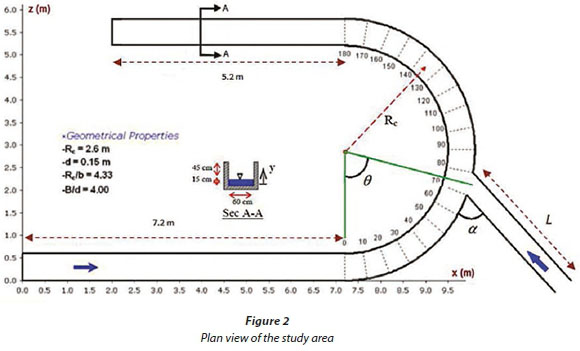
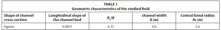
The bend used for the numerical solution is based on a 180° channel in the university of Tarbiat Modaress laboratory, which was used for Pirestani's experiments. The channel cross-section is a square with 0.6 m width and height. The input channel before the bend and output channel after the bend are 7.2 m and 5.2 m respectively. A 4-m long straight channel that was located 45° from the beginning of the bend with different angles (a) relative to the bend (30°, 60°, 90°, and 115°) was used as a tributary channel; the tributary channel's wall and bed were made of plexy glass (k_s=0.0001). The geometric characteristics of the main channel are presented in Table 1. The plan view of the considered confluence layout is presented in Fig. 2.

 

 

Numerical model: theory, assumption and boundary condition

The analytical equations governing the flow conditions are the Navier-Stokes equations used for turbulent viscous incompressible fluids: i.e., the continuity (1) and momentum (2) equations. Assuming a constant flow and regardless of the density changes these equations are as follows:

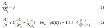
where: u is the average velocity, ρis the flow density, P is the total pressure, δis the Kronecker delta, x is the general distance dimension and pu_iu_jare known as the Reynolds turbulence stresses. These stresses are calculated by the Boussinesq approximation:

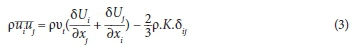
where: k is the turbulent kinetic energy and is defined by Eq. 4:

In order to solve Eq. 3, the main task is to determine the turbulent eddy viscosity (ν_t), which is obtained by the turbulent model. The K-ε model is the default turbulent model of the SSIIM1 software and determines ν_tas follows:

where: ε is the kinetic energy dissipation rate.

Boundary conditions for the Navier-Stokes equation are in many ways similar to the diffusion-convection equation, including boundary condition for inflow; outflow; water surface and bed/wall. Drichlet boundary conditions have to be given at the inflow boundary. This is relatively straightforward for velocity, but it is usually more difficult to specify the turbulence. It is then possible to use a simple turbulence model (ν_t = 0.11u'h or ν_t= 0.067u'h) to specify the eddy viscosity. Given the velocity, it is also possible to estimate the shear stress (τ) at the entrance bed. The turbulent kinetic energy K at the inflow bed is then determined using the following equation:

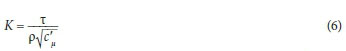
Given the eddy viscosity and K at the bed equation gives the value of εat the bed. If K is assumed to vary linearly from the bed to the surface then Eq. 5, together with the profile of the eddy viscosity, to calculate the vertical distribution of e, can be used.

The free surface is computed using a fixed-lid approach, with zero gradients for all variables. The location of the fixed lid and its movement as a function of time and the water flow field are computed using pressure and the Bernoulli algorithm. The algorithm is based on the pressure field. It uses the Bernoulli equation along the water surface to compute the water surface location based on a fixed point that does not move (in this study, downstream of the confluence).

The wall law for rough boundaries was used as a boundary condition for bed and wall:

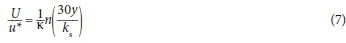
Here, the roughness is denoted k_s. In this study, for the bed effective roughness according to the Van Rijn equation is used; U and u* = velocity and shear velocity, respectively, k is a coefficient equal to 0.4 and y is distance from the wall to the centre of the cell.

Computational grid

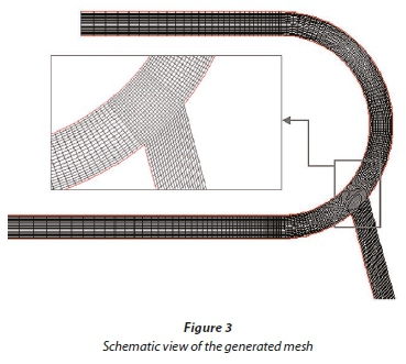
The SSIIM1 model is not capable of producing the desired mesh alone; therefore a mesh generator program was written in MATLAB for the study domain. The program is written in such a way that, based on user demand (by taking the number of nodes in the direction of the channel's length), width, tributary channel position and the tributary junction angle and length, it can produce the range of the field and its mesh. The program also uses a specific algorithm to set the mesh in such a way that smaller meshes are used in areas near the main channel wall, near the bend junction and in the tributary channel. Also, in order to reduce the computation time, in the upstream and downstream straight channels the mesh is set in such a way that when approaching the bend in the flow direction the mesh gets smaller. Figure 3 shows the mesh produced by this program. The 201x61x13 grid in x, y and z direction was chosen as the optimum mesh size for this research.

 

 

Model validation for simulating the flow pattern

First, the model is validated by comparing and analysing the numerical simulation results and the results of the tests carried out in the vertical junction of 2 straight channels and a simple bend (without junction). Then, by placing the junction channel in a 45° position from the beginning of the bend and using different junction angles in the bend, the flow pattern in the junction is studied.

Validating the flow in straight channel junctions

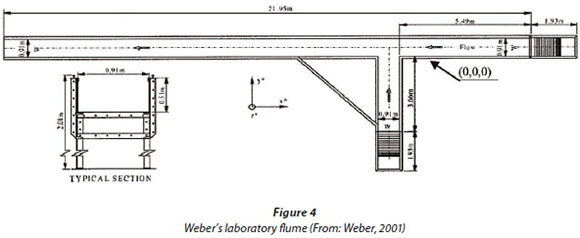
Weber et al.'s (2001) measurement results from Iowa University were used for validating the model for a 90° junction in straight channels. The length of the main channel and tributary channel of Weber's laboratory model were 21.946 m and 3.568 m, respectively (Fig. 4). The sub-channel is located 5.486 m downstream of the main channel. The main channel and sub-channel's width are both 0.914 m and the channel bed is completely horizontal. The coordinate system is as follows: the positive x direction is pointed upstream of the main channel, the positive y is in the tributary channel's direction and the positive z is in the upward direction. The origin of the coordinates is located at the upstream corner of the junction. The total discharge downstream of the main channel is 0.17 m³/s and the upstream depth and velocity are 0.296 m and 0.628 m/s respectively. The main channel's discharge upstream of the junction and the tributary discharge are 0.127 and 0.043 m³/s respectively. The discharge ratio (tributary discharge versus total discharge) is q*=0.25.

 

 

The model has a 225x44x12 grid in the x, y, and z directions, respectively. The cell heights were considered variable in the vertical direction and cells with smaller heights were chosen near the bed.

The longitudinal water surface profile calculated along the left bank, the centre line and the right bank of the main channel were compared with the laboratory data in Fig. 5. It is indicated that the numerical model can simulate the longitudinal water surface profile with good accuracy. The main difference is in the area between x/w = -1.3 to -2.4 and near the inner bank (y/w=0.167). In this area the model generally computes the water surface elevation to be greater than its actual value. This difference is due to the separation zone and the turbulent k-ε model's weakness in rotational flow areas, and possibly also water surface elevation measurement errors due to the intense turbulence of the flow.

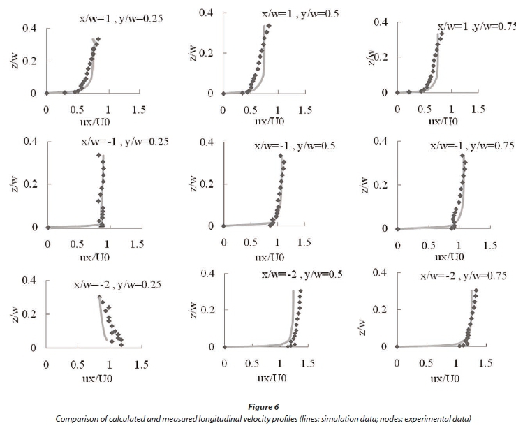
The comparative analysis between measured and calculated longitudinal velocity profiles in different sections of the main channel is shown in Fig. 6. The longitudinal velocity is non-dimensionalized by downstream longitudinal velocity Uo and x, y and z components are non-dimensionalized by width of the channel, w.

The results showed that the model had a relatively high accuracy in predicting velocity profiles. A remarkable difference is in section x/w= -2 and y/w=0.25 which is near the separation zone. This difference could be due to the weakness of K-ε model in the rotational zone. Weerakoon et al. (1991) pointed out that the K-εmodel has a weakness in separation zone size, and predicted dimensions of the separation zone that were lower than the actual value. In Fig. 7, comparison of the measured and simulated longitudinal velocity shows that the model predicted longitudinal velocity with 90% accuracy.

 

 

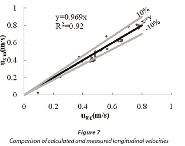
As can be seen from this figure, most of data are within the 10% error bands. Several points that are below -10% are in the separation zone, where, because of recirculation flow and weakness of the K-ε model, maximum error of flow pattern prediction occurred. Also, the root mean square error was 0.052 m/s for longitudinal velocity. The coefficient of determination and slope of regression line were 0.92 and 0.969, respectively. This indicates that the model can be applied for prediction of flow pattern in river confluences.

Validating the flow in the bend

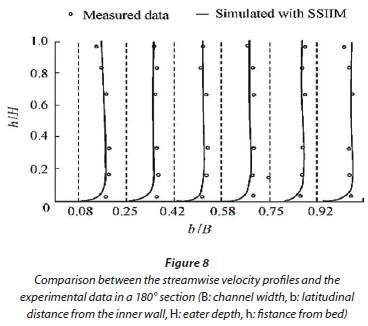
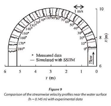
The model validation in the bend is based on the channel used in Pirestani's (2004) laboratory experiments. The bend consists of a 91x19x7 grid in the x, y, and z directions, respectively, which is introduced as the optimum mesh size in a 180° uniform bend. The length of the straight input channel before the bend and output channel after the bend are 7.2 m and 5.2 m, respectively. The channel bed and wall are made of plexy glass. The channel discharge is 30 L/s and the simulation of flow pattern is based on this discharge. In order to validate the numerical modelling, the results of modelling in a bend with a uniform width of 0.6 m were compared with Pirestani's laboratory results (shown in Figs 8 and 9). The results indicate that the velocity profiles calculated by the numerical model are in total agreement with the laboratory data and the numerical model is able to simulate the flow field in a uniform bend very well. They also show that the model is properly calibrated.

 

 

 

 

RESULTS

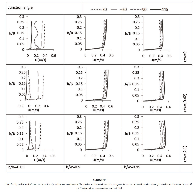
The effect of the junction angle on the vertical profiles of streamwise velocity in the main channel

Figure 10 presents a comparison of the vertical profiles of stream-wise velocity in 4 junction angles (30°, 60°, 90°, 115°), in 3 cross-sections (x/w=0, x/w=0.42 and x/w=2.1) and along 3 streamwise transects (b/w=0.05, b/w=0.5 and b/w=0.95). Except for the outer bank (b/w=0.05), in all the sections the velocity has increased by increasing the junction angle. Close to the outer bank (b/w=0.05) the velocity profiles are different from the other sections because of the existence of the separation zone. By increasing the junction angle the separation zone dimensions also increase and the return flow in the separation zone reduces the flow velocity. It can be seen in section x/w=0.42 that for junction angles 90° and 115° negative velocities occur in the outer bank.

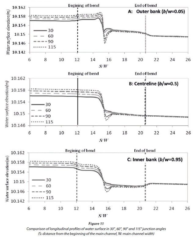
The effect of junction angle on water surface longitudinal profiles

In Fig. 11 the effect of 4 junction angles, 30°, 60°, 90° and 115°, on the longitudinal profiles of the water surface are shown. It is indicated that by increasing the junction angle the difference between the upstream and downstream water levels increases. The difference is more significant in the outer bank. By increasing the junction angle the amount of flow penetrating from the tributary to the main channel increases and the main channel's effective width decreases which leads to backwater occurring upstream.

The effect of junction angle on bed shear stress distribution

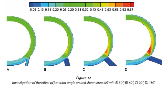
Examining the bed changes requires a combined study of the flow and bed sediment and their interactions. However by taking the bed shear stress into account, we can partly predict the erosion and sediment patterns for real streambeds. Figure 12 indicates the results of shear stress in junction angles 30°, 60°, 90° and 115°. It can be seen that by increasing the junction angle the maximum shear stress also increases. The maximum shear stresses for 30°, 60°, 90° and 115° are 0.44, 0.5, 0.61 and 0.7 N/m², respectively. By increasing the junction angle the separation zone's width increases and the effective width of the flow decreases which leads to an increase in the flow velocity and therefore the shear stress increases. The increase in the bed shear stress ultimately leads to excessive erosion downstream of the junction in the vicinity of the maximum shear region. By increasing the junction angle from 30° to 115° the maximum bed shear stress in the junction increases 59%.

 

 

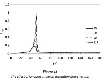
The effect of junction angle on secondary flow strength

The concept of secondary flow strength is used to evaluate dissipation rate of secondary flow in the channel bend. This is defined by Mosonyi and Gotz (1973) as follows:

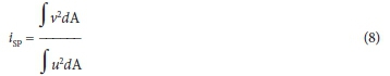
where: νis the mean lateral velocity, u is the mean longitudinal velocity in each of the available cells, and dA is the cross section of the cell. Figure 13 shows the spiral flow strength in 4 junction angles (30°, 60°, 90° and 115°); it is indicated that in all the simulated situations from the beginning of the bend to the intersection of the two flows, the secondary flow increases. This is in fact the area where the secondary flow is created due to the centrifugal force overcoming the longitudinal pressure gradient. Due to the entrainment of flow from the tributary channel to the main channel, and the increase of the transverse velocity in the junction, the numerator of Eq. 8 significantly increases. Figure 13 also indicates that the secondary flow strength reaches its maximum value in the junction and increasing the junction angle affects and increases the spiral flow.

 

 

CONCLUSIONS

In this research the SSIIM1 model was used to evaluate the effect of the tributary junction angle on the flow pattern in a 180° bend. By placing the tributary channel in a 45° position from the beginning of the bend, the effect of 4 junction angles (30°, 60°, 90° and 115°) was evaluated. The results showed that changing the junction angle affects the flow pattern. Evaluating the vertical velocity profiles showed that by increasing the junction angle the flow velocity also increases. The results showed that along the right bank and in the vicinity of the junction a separation zone occurs and by increasing the junction angle the separation zone dimensions increase.

Evaluating the water level profiles in the main channel's right bank, centreline and left bank indicated that increasing the junction angle increases the difference between the upstream and downstream water level and the difference is more significant along the right bank (near the junction). Increasing the junction angle increases the maximum shear stress; by increasing the junction angle from 30° to 115° the maximum bed shear stress in the junction increases 59%.

Because of the flow entrainment from the tributary channel to the main channel and the increase in the transverse velocity in the junction, the secondary flow strength in the main channel increases significantly. Increasing the junction angle also affects the spiral flow strength so that the maximum secondary flow strength occurs with a 115° degree junction angle.

 

REFERENCES

ALAMATIAN A and JAFARZADE MR (2010) Simulation of supercritical flood flow at the junction channels. 5^thNational Congress of Civil Engineering, 4-6 May 2010, Mashad, Ferdosi University, Iran.         [ Links ]

BAGHLANI A and TALEBBEYDOKHTI N (2013) Hydrodynamics of right-angled channel confluences by 2D numerical model. Iran. J. Sci. Technol. Trans. Civ. Eng. 37 (C2) 271-283.         [ Links ]

BARANYA S, OLSEN NRB and JOZSA J (2013) Flow analysis of river confluence with field measurements and rans model with nested grid approach. River Res. Applic. http://dx.doi.org/10.1002/rra.2718.         [ Links ]

BIRON PM, RAMAMURTHY AS and HAN S (2004) Three-dimensional numerical modeling of mixing at river confluences. J. Hydraul. Eng. 130 (3) 243-225. http://dx.doi.org/10.1061/(ASCE)0733-9429(2004)130:3(243).         [ Links ]

BRADBROOK KF, LANE SN, RICHARDS KS, BIRON PM and ROY AG (2000a) Large eddy simulation of periodic flow characteristics at river channel confluences. J. Hydraul. Res. 38 207-215. http://dx.doi.org/10.1080/00221680009498338.         [ Links ]

BRADBROOK KF, LANE SN, RICHARDS KS BIRON PM and ROY AG (2000b) Numerical simulation of three-dimensional, time-averaged flow structure at river channel confluences. Water Resour. Res. 36 (9) 2731-2746. http://dx.doi.org/10.1029/2000WR900011.         [ Links ]

CHEN SC and PENG SH (2006) Two-dimensional numerical model of two-layer shallow water equations for confluence simulation. Adv. Water Resour. 29 (11) 1608-1617. http://dx.doi.org/10.1016/j.advwatres.2005.12.001.         [ Links ]

DORDEVIC D and BIRON PM (2008) Role of upstream planform curvature at asymmetrical confluences - laboratory experiment revisited. In: Proc. 4^th Int. Conference on Fluvial Hydraulics - River Flow 2008 3 2277-2286.         [ Links ]

DORDEVIC D (2013) Numerical study of 3D flow at right-angled confluences with and without upstream planform curvature. J. Hydroinf. 15 (4) 1073-1088. http://dx.doi.org/10.2166/hydro.2012.150.         [ Links ]

GHOBADIAN R (2008) The study effect of tail water level changes on secondary currents at rectangular channels confluence with a three- dimensional model. In: 4^th National Congress of Civil Engineering, 1-3 May 2008, Tehran University, Tehran, Iran.         [ Links ]

HUNG JL, WEBER LJ and YONG GL (2002) Three-dimensional numerical study of flows in open-channel junctions flow. J. Hydraul. Eng. 128 (3) 268-280. http://dx.doi.org/10.1061/(ASCE)0733-9429(2002)128:3(268).         [ Links ]

MOSONYE E and GOTZ W (1973) Secondary currents in subsequent model bends. International Symposium on River Mechanics 1 191-201. Asian Institute of Technology, Bangkok, Thailand.         [ Links ]

PIRESTANI M (2004) Investigation on flow field and scouring at lateral intake in channel bends. PhD thesis, Islamic Azad University, South Tehran branch, Iran.         [ Links ]

RILEY JD and RHOADS BL (2012) Flow structure and channel morphology at a natural confluent meander bend. Geomorphology 163-164 84-98. http://dx.doi.org/10.1016/j.geomorph.2011.06.011.         [ Links ]

ROBERT MVT (2004) Flow dynamics at open channel confluent-meander bends. PhD thesis, University of Leeds, United Kingdom.         [ Links ]

WEERAKOON SB, KAWAHARA Y and TAMIA N (1991) Three dimensional flow structure in channel confluences of rectangular section. Proceedings of the 24^th Congress of the International Association of Hydraulic Research A, 9-13 September 1991, Madrid. 373-380.         [ Links ]

WEBER LJ, SCHUMATE ED and MAWAR N (2001) Experimental on flow at a 90° open-channel junction. J. Hydraul. Eng. 127 (5) 340-350. http://dx.doi.org/10.1061/(ASCE)0733-9429(2001)127:5(340).         [ Links ]

YANG QY, LIU TH, LU WZ and WANG XK (2013) Numerical simulation of confluence flow in open channel with dynamic meshes techniques. Adv. Mech. Eng. 2013 (860431) 1-10. http://dx.doi.org/10.1155/2013/860431.         [ Links ]

 

 

Received: 4 December 2014
Accepted in revised form 11 November 2015

 

 

* To whom all correspondence should be addressed. +989188332489; e-mail: Rsghobadian@gmail.com