Investigation into increasing short-duration rainfall intensities in South Africa

 

 

JA Du Plessis^*; GJ Burger

Department of Civil Engineering, University of Stellenbosch, P/Bag X1, MATIELAND 7602, South Africa

 

 

---

ABSTRACT

Extreme storms in South Africa and specifically in the Western Cape have been responsible for widespread destruction to property and infrastructure, even leading to displacement and death. The occurrences of these storms have been increasingly linked to human-induced climate change that is expected to cause more variable weather. Studies on climate circulation models for future climate conditions project that rainfall in the Western Cape and wider South African region is to become more intense and extreme. Sub-daily rainfall for 3 stations in the Western Cape and 4 stations in the rest of South Africa were analysed in order to determine if any trends towards more intense and extreme rainfall are observed and whether the trend is unique to the Western Cape or indicates a wider trend. This study explores this expectation by using historical short-duration rainfall (less than 24 h) for 7 stations in the Western Cape and South African region. Digitised autographic and automatic weather station 5-min rainfall data were combined to extend the effective record length. Both the magnitude and frequency of occurrence of rainfall events were analysed to assess if rainfall intensities are showing any evidence of increasing over time. For the magnitude of rainfall events, extreme value theory was applied to non-stationary sequences, using both a parametric and non-parametric approach for both event maxima and peaks over threshold modelling. The frequency analysis entailed measuring the frequency of exceedance of rainfall events over a certain threshold value. Both the magnitude and frequency analysis indicated that the combination of the two record types influenced the results of some of the stations, while the others showed no consistent evidence of changing rainfall intensities. This led to the conclusion that, from the available observed short-duration record, no evidence was found of trends or indications of changes in rainfall intensities.

Keywords: climate change, short duration rainfall, extreme value theory, non-stationary

---

 

 

INTRODUCTION

Developments in climate sciences over the past 20 years are attributing the increasing occurrence of extreme weather events like droughts and floods to changing climate conditions as a result of increases in atmospheric greenhouse gas concentrations caused by rapid human development since the industrial age. In particular, this change in climate is expected to change the characteristics of rainfall, particularly the magnitude and frequency of occurrence of rainfall events (Trenberth et al., 2003; Holtzhausen, 2006; Benhin, 2006).

Observations on rainfall and runoff in South Africa already show great inter-annual variability that are prone to cause either drought- or flood-related weather events (Schulze, 2003). In particular, the Western Cape Province has been host to a number of extreme rainfall events in the past decade causing displacement of people, deaths, damage to property and infrastructure (Holloway et al., 2010). To improve decision making in this regard, an understanding of the mechanisms at work is required and a number of critical questions can be asked: What role does climate change play with the frequency and intensity of these storms in South Africa? Are design practices used to anticipate and design for storms, based on the stationarity (i.e. assuming that the mean climate conditions will remain the same over time) of the climate, still adequate? If not, is this a phenomenon unique to the Western Cape or is it observed in other parts of South Africa?

Whilst studies on observed rainfall records conducted for the Western Cape, wider South and Southern African region do not indicate an overall regional trend in rainfall behaviour, there seems to be some consensus over a tendency towards more extreme and variable rainfall (Fauchereau, 2003, Groisman et al., 2004; Midgley et al., 2005; Kruger, 2006; New et al., 2006; Schulze et al., 2011; Hoffmann et al., 2011).

Most of these studies however focussed on daily or 24-h rainfall. Design storm durations for some catchments, especially in urban areas, are often shorter than 24 h and require rainfall measured over shorter durations. Van Wageningen and Du Plessis (2007), analysing 5-min rainfall data for the Molteno reservoir rainfall station in Cape Town in the Western Cape over the period 1961-2003, found that the occurrence of rainfall events decreased from the 1990s, while the average magnitude of the 5-min events increased over the same period, indicating increasing intensities. It was uncertain if these results were unique to the single station used in the analysis, or indicated greater spatial significance, but the results support the contentions of Trenberth et al. (2003), who lay out the reasons for fewer rainfall events but with greater intensities that result from a warming climate.

The aim of the research presented in this paper is to expand on the work done by Van Wageningen and Du Plessis (2007), by analysing short-duration rainfall for more rainfall stations in order to ascerain whether there are any indications of a wider regional pattern to increasing rainfall intensities in the Western Cape and whether similar trends are observed in the rest of the country.

Extreme value theory

Stormwater systems are designed to effectively drain rain-induced runoff for at least some extreme storm events. Intensity duration frequency (IDF) curves are typically used in stormwater design to determine a specific rainfall intensity for a corresponding storm duration value according to a specific probability of occurrence. IDF curves are typically derived by fitting statistical distributions to different storm duration rainfall data and obtaining the specific intensity design levels for the relevant return periods. Extreme storm events are, by definition, rare and show different behaviour to the overall rainfall behaviour. The use of improper statistical distributions to model extreme events could lead to the underestimation of an event which could lead to increased socio-economic costs through poor design, and loss of infrastructure and human life.

Classical extreme value theory can be divided into 2 branches: block maxima modelling and peaks over threshold modelling. Block maxima modelling is very commonly applied in hydrological design, typically by selecting the maximum value that occurred over an annual period, hence the name annual maxima series (AMS). The generalised extreme value distribution (GEV) is the basic distribution derived for block maxima series. The GEV, in cumulative probability form, is given as (Coles, 2001):

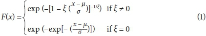
where: μ, σ and ξ are the location, scale and shape parameters, respectively, for an independent identically distributed AMS series x. The AMS is the most widely applied method and recommended in South African hydrological contexts (Van Bladeren et al., 2007). It is simple to apply and there is good confidence in the independence of events. However, what happens if a number of large events occur within the same year? According to the AMS method, only the largest event in the year will be selected, while the other large events will be ignored and the method potentially loses valuable information.

The peaks over threshold (POT) method overcomes this challenge by selecting all events above a certain value, ensuring that a larger sample of large events is used for analysis. The main benefit is that more data points can be used for analysis than is the case for AMS. The generalised Pareto distribution (GPD) has been shown to be the adequate distribution for POT series, with the cumulative probability form (Coles, 2001):

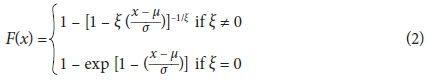
where: u is the threshold, x is an independent identically distributed variable with the other parameters the same as for the GEV. The greatest challenge of the GPD/POT methodology is the selection of the threshold value, as too high a threshold increases the variance of the calculated values, but too low a threshold undermines the assumption of independent events (Wang, 1991; Coles, 2001). As of yet, no objective method exists to select the threshold value (Katz et al., 2005), though a number of methods have been suggested that could aid with the selection of the threshold. Interpretative plots like the Hill and mean residual life plot have been suggested, but these are often difficult to interpret and also suffer from a degree of subjectivity (Coles, 2001). Claps and Laio (2003) and Ben-Zvi (2009) have suggested raising the threshold from a very low level until some goodness of fit criteria are met. In spite of these apparent difficulties, there is room for the application of GPD/POT methodology given the benefit of additional data points and the consideration of only the most extreme events.

One of the problems in current engineering design is the underlying assumption of the stationarity of the climate, that is, that future conditions will remain the same as current conditions. Typically, when an extreme value distribution is applied to a dataset, it is assumed that the series of extremes are independent and identically distributed, that is, the values are not dependent on each other and that they all have the same common distribution. Although not explicitly stated, an example of this assumption used in civil engineering design is seen in the Drainage Manual (SANRAL, 2006), where it is assumed that the selected fitted distribution will remain the same for the determined return periods. With climate change possibly influencing the characteristics of rainfall over time, this assumption is not necessarily valid.

One means to address this assumption is by testing for possible non-stationarity when using extreme value theory. This can be done by applying parametric or non-parametric methodology. The parametric method models extreme value distributions by applying some model to the parameters of the distribution, like a linear time model applied to the location parameter (Coles, 2001):

where: β₀ and β₁ are the intercept and slope values and t is a time variable value. The time value can, for example, represent the number of years in the case of an AMS. In this way, the distribution varies over each year, in contrast to identically distributed cases.

The non-parametric method works on the basis that, if a dataset is stationary, the return values of the distribution must stay constant over time. The data is divided into equal time periods that can either overlap or be distinct; a distribution is then fitted to each time period, and the estimated return values of the corresponding specific return period are plotted. If the values show any trend or large deviance over time, it could indicate possible non-stationarity. Studies applying non-parametric methods do not provide explicit criteria on a minimum length of the time period, which ranged between 20 to 30 years and made use of return values for lower return periods ranging between 10 and 20 years (Brath et al., 2001; Begueria et al., 2011).

Whilst a number of international studies have investigated the application of non-stationarity in extreme value theory for hydrological data (Begueria et al., 2011; Brath et al., 2001; Jakob et al., 2011; Katz et al., 2005; Li et al., 2005; Park et al., 2011), no studies in a South African context could be found. In light of this, and possible increases in rainfall intensities in the Western Cape and wider South Africa, there is room to apply non-stationary extreme value theory to rainfall data in South Africa.

Data selection and processing

Short-duration rainfall (SDR) data were obtained from the South African Weather Service (SAWS) and consisted of 2 record types: digitised autographic rainfall data up to approximately 1992 and 5-min rainfall data from automatic weather stations (AWS) since 1994. The autographic record underwent an interpolation and summation process to convert the data into equivalent 5-min intervals of the AWS data, in order to combine the two record types and extend the effective record length.

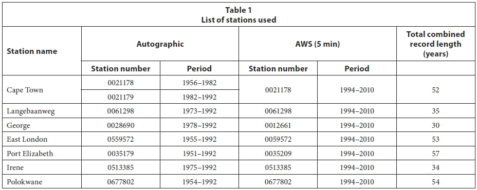
Although 412 stations were initially selected, numerous errors and data quality issues were encountered, especially with the digitised autographic data; consequently, many stations had to be disregarded. Seven stations, listed in Table 1, were selected for further analysis.

Data analysis

SDR data was further processed into storm duration data for durations 5, 10, 15, 30, 45, 60 and 90 min and 2, 4, 8, 12, 18 and 24 h, as typically used with intensity duration frequency (IDF) curves. Analysis was divided into 2 sections, the magnitude and the frequency of occurrence of rainfall events. The magnitude analysis focussed on the amount of rainfall calculated over the aforementioned storm durations using non-stationary sequences on extreme value distributions in order to determine if rainfall events are becoming more extreme over time. The frequency analysis focussed on the number of occurrences of 5-min readings exceeding a certain threshold, in order to ascertain if more rainfall events are occurring.

The magnitude analysis consisted of the application of extreme value distributions to non-stationary sequences for the seven selected stations. The analysis consisted of both a parametric non-stationary (PNS) and a non-parametric non-stationary (NPNS) approach, as discussed above.

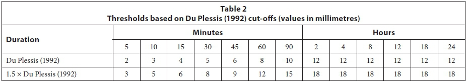
Both block maxima and peaks over threshold approaches were used, with the GEV distribution in conjunction with an annual maxima series (AMS) and the GPD for the peaks over threshold series. For the POT approach, 3 methods were used to determine the threshold. Two approaches were based on values from Du Plessis (1992) as highlighted in Table 2, which ensures that the top rainfall peaks will be selected for the Cape Town area.

The third approach was based on a methodology where the shape parameter for the data set, consisting of the number of exceedances above a selected threshold value, was calculated. This data set (number of occurrences) was systematically increased as a result of an increased threshold value. This approach resulted in a range of shape parameters, one associated with each data set represented by a range of exceedances. The regions where the shape parameters appear to be most stable (no large deviations), were identified and the corresponding threshold value closest to the stable region selected for further calculation.

Extreme value distribution parameters were estimated using the maximum likelihood method by means of a modified version of the ismev package in the R programming language. The maximum likelihood method estimates the parameters through optimisation techniques and was also used to estimate confidence levels in both the parameters and the return levels.

Peak values were selected on the basis that peak events from a rainfall event must be separated by at least 24 h of zero rainfall, in order to ensure a measure of independence between peak events used in the POT approach.

Once the threshold value was identified per storm duration, a data set, consisting of the number of exceedances above the selected threshold value, was used for further analysis. These data were analysed using both the PNS and NPNS methodologies.

For the PNS method, a linear model was applied to each parameter of the respective distribution used. For the GPD, only the ξ and σ parameters were tested as the threshold was already selected and was kept constant over time. The significance of each parameter's model was selected by applying a t-test (based on the t-distribution) to the slope (β₁) for a 95% confidence level. If any linear time parameter showed a significant fit, then the parameter was incorporated into the distribution. The non-stationary model (with linear time parameters) would then be compared to a stationary model (with constant parameters) by using the deviance statistic, based on the log-maximum likelihoods of each model calculated from the maximum likelihood method. The deviance statistic is given as (Coles, 2001):

where: D is the deviance statistic and l₀(M₀) and l₁(M₁) is the log-maximum likelihood for the less and more complicated model respectively. The more complex model, M₁, is accepted if D > , where is the 95% quantile for the chi-square distribution and where k is the difference between the numbers of parameters of the models. The total number of significant non-stationary fits over all storm durations was recorded.

The NPNS analysis is based on fitting EVT distributions to the storm rainfall events identified over a specific period (say 20 years, 1990 to 2010) and then changing that period with 1 year (still 20 years, but now from 1991 to 2011) to produce a 1-year moving window and obtaining the storm rainfall in mm for the corresponding return period, similar to a moving average calculation. Three window periods, 15, 20 and 25 years, were used and storm rainfall (mm) for return periods 5, 10 and 20 years was calculated. The range of window and return periods was used to determine if results are generally consistent. Return periods were kept low since the variance for large return periods became extremely large.

For a specific distribution, and storm duration, a series of storm rainfall values for a specific return period would be produced over the range of window periods. Linear regression would be applied to the series of storm rainfall values for a specific window and return period. The significance of the slope of the regression line would be measured with the t-test for a 95% level of significance. For all combinations of return and window periods, the number of significant slopes and corresponding sign of the slopes would be recorded. This procedure is applied to all storm durations for both the GEV distribution and GPD.

Frequency analysis

The frequency analysis used a modified approach to that used by Van Wageningen and Du Plessis (2007). All 5-min rainfall events exceeding threshold values 0.5, 1 and 2 mm for each year were plotted for any visible trends. Rainfall above a threshold value was used instead of using all the data, as in Van Wageningen and Du Plessis (2007), since the interpolation technique for the autographic data includes low rainfall values (< 0.2 mm) interpolated over long durations, resulting in extremely low and arguably unrealistic rainfall values that will be counted as an event.

 

RESULTS

The PNS method produced significant non-stationary models for the GEV distribution, while no significant fits were observed for the regressions applied to the parameters derived from the GPD for all three threshold methods. Table 3 indicates which storm duration data produced significant non-stationary distributions and which parameters fitted over the relevant storm durations. The parameters listed in Table 3 indicate all the relevant fitted non-stationary parameters which varied per specific storm duration.

 

 

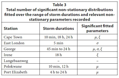
Non-stationary fits were typically erratic over the range of storm durations, as in the case of Cape Town, East London, Irene and Polokwane, where no pattern of non-stationary fits was observed, or in the case of Langebaanweg, where no significant non-stationary fits were recorded. Only George and Port Elizabeth indicated some consistency as a whole range of consecutive storm durations showed non-stationary fits.

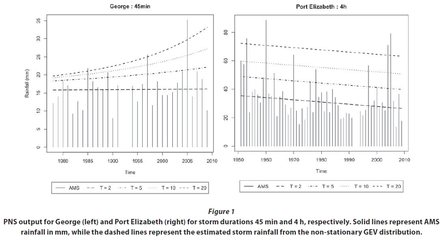
The results for George and Port Elizabeth were investigated further. George's significant NS results were for all storm durations longer than 45 min, while those for Port Elizabeth were for storm durations longer than 4 h. All non-stationary results for George produced increasing storm rainfall values, with 6 of the 9 durations producing positive coefficients for the slopes for the shape parameter, ξ, indicating that the storm rainfall become more extreme over time. Figure 1 (left) illustrates a typical output generated from the analysis. Although the parameters are estimated linearly, the effect of the shape parameter on the storm rainfall has a non-linear effect over time. In contrast to George's results, all Port Elizabeth's results produced decreasing storm rainfall estimates with time, with only the location parameter, μ, indicating non-stationarity. Figure 1 (right) illustrates a typical output for Port Elizabeth.

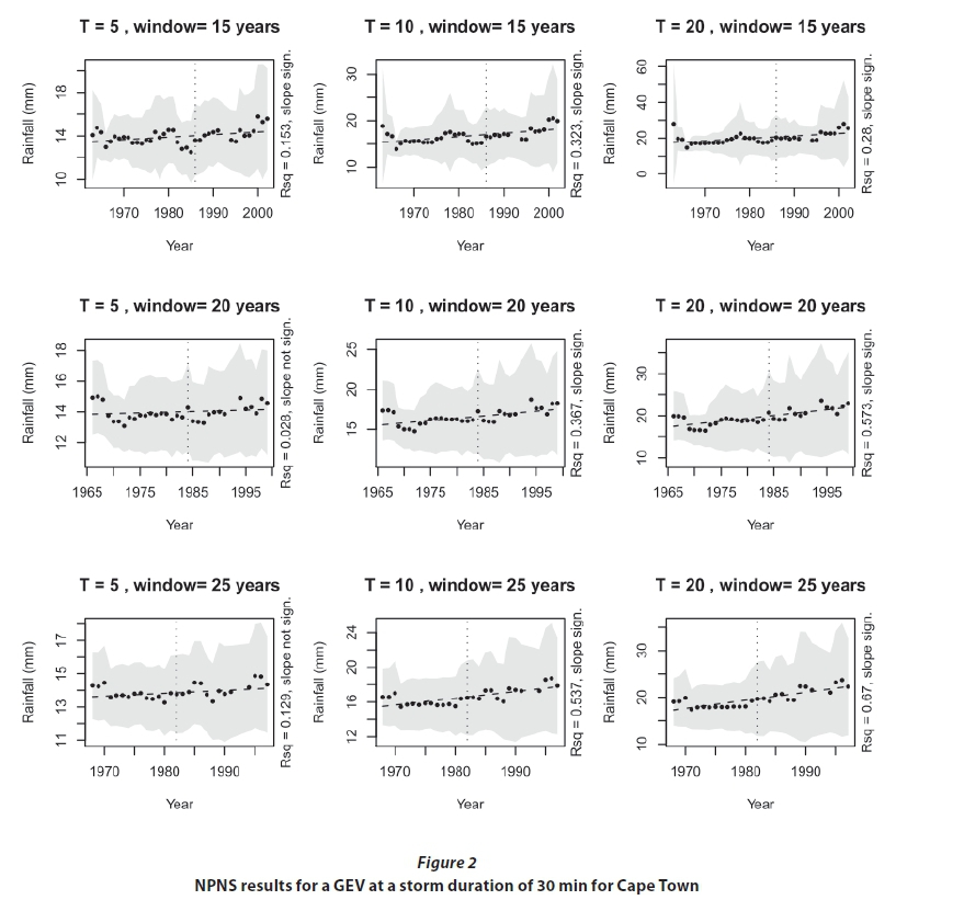
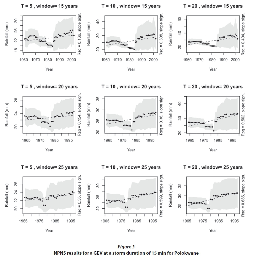
For the NPNS method, for each storm duration, 9 individual results were produced for each combination of the return period and window period per distribution. Figure 2 displays an example of the results of one storm duration for the GEV distribution. For each of the 9 instances, the slope of the line and the sign of the slope of the line were recorded. Positive slopes would naturally indicate increasing magnitudes over time, while negative slopes would indicate decreasing magnitudes.

Results for the GEV indicated that George and Polokwane produced strong positive trends, Port Elizabeth produced negative significant results for durations greater than 30 min, while the other stations produced varying signs for the slopes. Cape Town generally produced positive slopes, especially for durations between 15 and 45 min, East London produced positive slopes, especially for durations between 30 min and 8 h. Langebaanweg produced negative slopes for durations between 30 min and 8 h and very short and very long durations produced positive slopes. The results for Irene showed both positive and negative slopes, therefore indicating no overall trend.

Results of the GPD were more complicated, as 3 different threshold values were involved, but were generally in agreement with those of the GEV, although more amplified. Many stations produced up to 9 significant slopes for a number of durations. The sensitivity of the GPD to the threshold was also portrayed, where the three threshold selection methods produced large differences in some cases.

East London, Port Elizabeth, Irene and Polokwane showed indications of a change in slope with the change in record methodology from autographic to AWS at about 1994. Figure 3 presents a typical example of this (Polokwane), in which all of the window and return periods indicate a decrease in storm rainfall until approximately 1993/94 when the change in recording methodology occurred, after which the storm rainfall start to increase again. Though the regression indicates that the slope was significant, the actual storm rainfall values reflect something different. The resulting output of each storm duration for each distribution was visually investigated to assess if any slope changes occurred with the change in record.

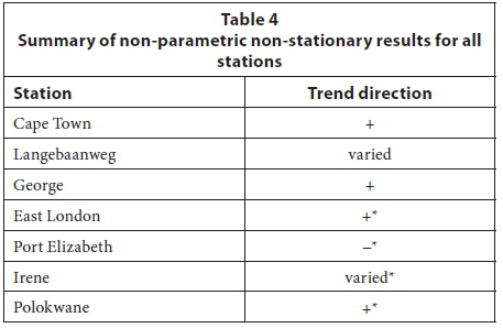
For both the GEV and GPD distributions, East London, Polokwane and Port Elizabeth showed changes of slope sign at the change of record, while a change at Irene was noted for the GPD distribution for all three thresholds. Since George used a shorter record length than the other stations, this influence could not be assessed with the graphs. Cape Town and most of the durations at Langebaanweg did not produce evidence of a change in slope at the change in the record type. The results of NPNS analysis for both the GEV and GPD are summarised in Table 4. The direction of the trends is indicated by either '+' for an increasing or '−' for decreasing storm rainfall over time. The possible influence of the change in record at the stations is indicated by '^*'.

 

 

Frequency analysis

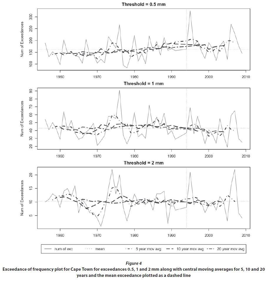
The frequency analysis recorded the number of exceedances above the thresholds 0.5, 1 and 2 mm per year for the complete 5-min dataset for all stations. Moving averages of 5, 10 and 20 years were fitted to the exceedances and plotted graphically, as illustrated in Fig. 4 for Cape Town. In Fig. 4 the light grey line represents the number of exceedances of the threshold per year, while the darker dashed lines represent the 5-, 10- and 20-year moving averages. The dotted horizontal line represents the mean number of exceedances. Also note the vertical dashed line in light grey at approximately 1994, representing the change in record type.

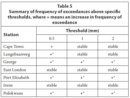
For a low threshold of 0.5 mm, exceedances increased from the 1990s at most stations, while thresholds of 1 and 2 mm generally produced similar increases for the stations in George, Polokwane and Port Elizabeth, or produced little change or smaller increasing trends at the other stations. The most likely reason for the increasing trends, especially for a low threshold, is the change of record type during the 1990s, and this is possibly because the digitised autographic data is unable to reflect very low rainfall values with the same degree of accuracy as the AWS data. This is supported by some stations producing few or slight changes for higher threshold values. Consequently, more weight is given to the higher threshold values. The results of the frequency analysis are summarised in Table 5. Positive and negative trends over time are indicated by '+' and '−', respectively, while the possibility of the influence of the record change is indicated by '^*'.

 

 

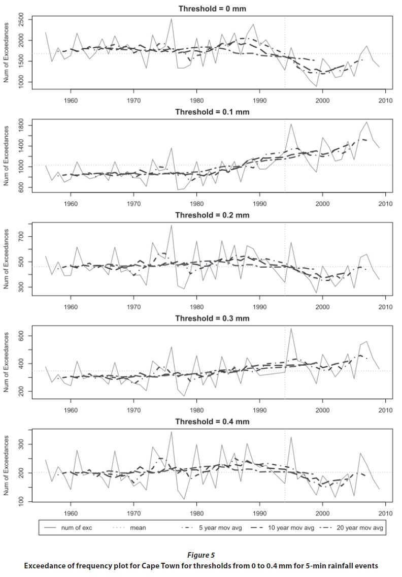
The importance of the aforementioned selected threshold values is illustrated in Fig. 5. In each sub-figure, the number of events exceeding the threshold value (indicated above each sub-figure) is shown. The threshold ranges from 0 (no threshold, i.e. all events) to 0.4 mm, increased by 0.1 mm increments. If no threshold is applied (top graph in Fig. 5), and therefore all rainfall events in 5 min are recorded, a clear drop in the number of exceedances is noticed from the 1990s, which is similar to the results of Van Wageningen and Du Plessis (2007). However, with a slight adjustment to an exceedance threshold level of 0.1 mm, the number of exceedances increased significantly after the 1990s. When the threshold is raised to 0.2 mm, a drop is again noticed from the 1990s. This pattern repeats itself for each slight adjustment of the threshold, although becoming weaker with each increase of the threshold value. The sensitivity of the number of exceedances to the slight increments of the threshold is explained by the nature of the autographic and AWS data. The autographic data consisted of interpolated values that were often very low (< 0.2 mm) and these values are then counted as events for the frequency analysis. In addition, the AWS only measures data in 0.2 mm increments and will therefore not record rainfall of less than 0.2 mm in 5 min as an event. For this reason the two datasets cannot be used for these low threshold values. With larger weight being given to the higher (0.4 mm) threshold value, it is clear from Fig. 5 that no definite pattern can be observed regarding the increase or decrease in the number of 5-min rainfall events.

The data used in Van Wageningen and Du Plessis (2007) for Molteno station in Cape Town were obtained for comparison, and a number of very low rainfall values (< 0.2 mm) were observed in this record for data before 1994. This seems to indicate that interpolation techniques similar to those used in this project were applied for the data supplied to Van Wageningen and Du Plessis (2007). The similarity between the results of Van Wageningen and Du Plessis (2007) and the zero threshold result in Fig. 5 indicate that the move from autographic to tipping bucket gauges is most likely the main cause of apparent changes in frequency and not any eccentricity in natural cycles (Van Wageningen and Du Plessis, 2007).

 

CONCLUSIONS

Both the magnitude and frequency analysis indicated that the data quality and change in recording methodology had a strong influence on many of the results. The only stations producing significant results for both magnitude and frequency analyses were George and Port Elizabeth, but there are strong indications that the change in the method of recording had an influence on the results. Of the remaining stations, those from the Western Cape, i.e., Cape Town and Langebaanweg, produced no significant PNS results, while showing some indication of changing storm rainfall over time with the NPNS. The frequency analysis for these stations did not indicate any visible trends in frequency of events either.

This leads to the conclusion that with the available short-duration rainfall record, consisting of mostly unreliable autographic data and a too short AWS dataset, no clear or significant evidence supporting increasing intensities consistent with the theories about the likely effects of projected changes in climate, or any other change in rainfall, was found regarding both the magnitude and frequency of occurrence.

Recommendations

Midgley et al. (2005) and Schulze et al. (2011) stated that climate change is more likely to cause seasonal shifts than changes in annual behaviour. As this research did not investigate seasonal effects in detail, possible seasonal trends for both magnitude and frequency should be studied further.

The limited amount of reliable digitised autographic data available in South Africa makes current short-duration rainfall related studies extremely difficult and it is recommended that for future studies only AWS data is used, which provide less opportunity for error in comparison to digitised data.

The application of the parametric non-stationary approach was limited to linear models. More complex models like quadratic and covariate models, which include seasonal, ENSO or similar sea surface temperature anomalies, as well as sunspot cycles, should be further investigated.

 

REFERENCES

BEGUERIA S, ANGULO-MATINEZ M, VICENTE-SERRANO SM, LOPEZ-MORENO JI and EL-KENAWY A (2011) Assessing trends in extreme precipitation events intensity and magnitude using non-stationary peaks-over-threshold analysis: A case study in Northeast Spain from 1930 to 2006. Int. J. Climatol. 31 (14) 2102-2114.         [ Links ]

BENHIN J (2006) Climate Change and South African Agriculture: Impacts and Adaptation Options. Centre for Environmental Economics and Policy in Africa (CEEPA), University of Pretoria, South Africa. ISBN 1-920160-21-3.         [ Links ]

BEN-ZVI A (2009) Rainfall intensity-duration-frequency relationships derived from large partial duration series. J. Hydrol. 367 (1-2) 104-114.         [ Links ]

BRATH A, CASTELLARIN A and MONTANARI A (2001) At-site regional assessment of the possible presence of non-stationarity in extreme rainfall in northern Italy. Phys. Chem. Earth, Part B: Hydrol. Oceans Atmos. 26 705-710.         [ Links ]

CLAPS P and LAIO F (2003) Can continuous streamflow data support flood frequency analysis? An alternative to the partial duration series approach. Water Resour. Res. 39 (8) 1216-1227.         [ Links ]

COLES S (2001) An introduction to Statistical Modeling of Extreme Values. Springer-Verlag, London.         [ Links ]

HOLLOWAY A, FORTUNE G and CHASI V (2010) RADAR Western Cape 2010. Crede Communications, Cape Town.         [ Links ]

HOLTZHAUSEN L (2006) Climate change: The last straw for communities at risk? The Water Wheel 5 (1) 17-21.         [ Links ]

JAKOB D, KAROLY DJ and SEED A (2011) Non-stationarity in daily and sub-daily intense rainfall - part 1: Sydney, Australia. Nat. Hazards Earth Syst. Sci. 11 (8) 2263-2271.         [ Links ]

KATZ RW, BRUSH GS and PARLANGE MB (2005) Statistics of extremes: Modeling ecological disturbances. Ecology 86 (5) 1124-1134.         [ Links ]

LI Y, CAI W and CAMPBELL EP 2005, Statistical modeling of extreme rainfall in southwest Western Australia. J. Clim. 19 (6) 852-863.         [ Links ]

MIDGLEY GF, CHAPMAN RA, HEWITSON B, JOHNSTON P, DE WIT M, ZIERVOGEL, G MUKHEIBIR P, VAN NIEKERK L, TADROSS M, VAN WILGEN BW, KGOPE B, MORANT PD, THERON A, SCHOLES RJ and FORSYTH GG (2005) A status quo, vulnerability and adaptation assessment of the physical and socio-economic effects of climate change in the Western Cape. ENV-S-C 2005-073, CSIR Environmentek, Stellenbosch.         [ Links ]

PARK J, KANG H, LEE YS and KIM M (2011) Changes in the extreme daily rainfall in South Korea. Int. J. Climatol. 31 (15) 2290-2299.         [ Links ]

SCHULZE RE, HEWITSON BC, BARICHIEVY KR, TADROSS MA, KUNZ RP, HORAN MJC and LUMSDEN TG (2011) Methodological approaches to assessing eco-hydrological responses to climate change in South Africa. WRC Report No. 1562/1/10, Water Research Commission, Pretoria.         [ Links ]

TRENBERTH KE, RASMUSSEN RM and PARSONS DB (2003) The changing character of precipitation. Bull. Am. Meteorol. Soc. 84 (9) 1205-1217.         [ Links ]

VAN BLADEREN D, ZAWADA PK and MAHLANGU D (2007) Statistical based regional flood frequency estimation for South Africa using systematic, historical and palaeological data. WRC Report No. 1260/1/07. Water Research Commission, Pretoria.         [ Links ]

VAN WAGENINGEN A and DU PLESSIS JA (2007) Are rainfall intensities changing, could climate change be blamed and what could be the impact for hydrologists? Water SA 33 (4) 571-574.         [ Links ]

 

 

Received 30 November 2012
Accepted in revised form 9 April 2015

 

 

* To whom all correspondence should be addressed: e-mail: jadup@sun.ac.za