Modelling mid-span water table depth and drainage discharge dynamics using DRAINMOD 6.1 in a sugarcane field in Pongola, South Africa

 

 

M Malota^{I, II}; A Senzanje^{I, *}

^ISchool of Engineering, University of KwaZulu-Natal, Pietermaritzburg, South Africa
^IIDepartment of Water Resources Management and Development, Mzuzu University, Mzuzu, Malawi

 

 

---

ABSTRACT

Determining optimal subsurface drainage design parameters through monitoring of water table depth (WTD) and drainage discharge (DD) at various combinations of drain depth and spacing is expensive, both in terms of time and money. Thus, drainage design simulation models provide for a simplistic and cost-effective method of determining the most appropriate subsurface drainage design parameters. In this study, the performance of the DRAINMOD model (Version 6.1) in predicting WTDs and DDs was investigated for a 32 ha sugarcane field in Pongola, South Africa. Water table depths were monitored in 1.7 m deep piezometers installed mid-way between two drains by using an electronic dip meter with a beeper, while DDs were measured at drain lateral outlet points, using a bucket and a stop watch. Both WTDs and DDs were monitored from September 2011 to February 2012. Results of the DRAINMOD model evaluation in predicting WTD, during calibration period, showed that there was a very strong agreement between simulated and observed WTDs with a goodness-of-fit (R²) of 0.826 and a mean absolute error (MAE) of 5.3 cm. Similarly, simulated and observed DDs during the model validation period also showed very strong agreement, with an R² value of 0.801 and an MAE of 0.2 mm∙day^-1. Results of simulated WTDs at various combinations of drain depth and spacing indicated that in clay soil a WTD of 1.0 to 1.5 m from the soil surface can be achieved by installing drain pipes at drain spacing ranging from 25 to 40 m and drain depth between 1.4 and 1.8 m. On the other hand, in clay-loam soil, the same 1.0 to 1.5 m WTD can be achieved when the drain pipes are installed at drain depths ranging from 1.4 to 1.8 m and corresponding drain spacing ranging from 55 to 70 m. Based on these results, it was concluded that DRAINMOD 6.1 can reliably be used as a subsurface drainage design tool in the Pongola region. This would simplify the design of subsurface drainage systems and the formulation of subsurface drainage design criteria for different crops and soil types found in the area and possibly throughout South Africa.

Keywords: drain depth; drain spacing; Hooghoudt's equation; model performance; saturated hydraulic conductivity; steady state conditions

---

 

 

INTRODUCTION

The soil system is one of the most complex natural systems, primarily due to great variations of non-linear processes occurring within it (Wang et al., 2006). For instance, infiltration is partitioned on the soil surface into percolation, storage and groundwater recharge. All these processes occur at different rates (Romano and Palladino, 2002; Bastiaanssen et al., 2007). In agricultural crop production systems, the main emphasis is on maintaining groundwater table depths below the crop root zone depth (Horton and Kirkham, 1999; Ritzema et al., 2006). This ensures sustaining a good balance of soil air, water and temperature within the root zone (Shultz et al., 2007). According to Smedema and Ochs (1998) and Vandersypen et al. (2007), such soil conditions are sustainably achieved by installing subsurface drainage systems in agricultural lands. The challenge, however, is how to accurately determine an optimum combination of drain depth, spacing and drainage discharge that can best suit a given cropping system (Bos and Boers, 2006; Shultz et al., 2007).

Historically, optimization of the aforementioned parameters has been achieved through the physical monitoring of groundwater table depth at varied drain depth and spacing combinations (ASAE Standards, 1999). However, this method is expensive in terms of setting up the experimental plots. In addition, the time requirements for this method make it unsuitable for agricultural water management systems in that they require timely decisions (FAO, 2007). It is therefore not surprising that the use of computer-based drainage design simulation models such as DRAINMOD (Skaggs 1978, 1980), SaltMOD (Oosterbaan, 2000) and WaSim (Hess et al., 2000) are increasingly becoming more reliable in subsurface drainage design.

In the South African context, nearly a quarter of the total 1.3 million ha under irrigation is affected by soil salinisation and waterlogging and reclamation plans need to be effected (Backeberg, 2000). Unfortunately, the problem appears to be escalating (DWAF, 2004). Furthermore, there are no generally well-established and accepted subsurface drainage design criteria in South Africa. The current drainage design approaches were developed in an ad hoc manner more than 26 years ago (Van der Merwe, 2003). There is evidently an urgent need to address the problem in a more cost-effective manner.

This study focused on assessing the applicability of the DRAINMOD model as a tool for subsurface drainage design in South Africa. The study was conducted in a sugarcane field in Pongola, South Africa.

Description of the DRAINMOD model

The DRAINMOD model is one of the most widely-applied models in subsurface drainage system design (Skaggs, 1976, 1978, 1980; Wang et al., 2006; FAO, 2007). According to Skaggs (1978), the model uses functional algorithms to approximate the hydrological components in soils with shallow water tables. Inputs to the model are weather data, soil data and crop information (effective root zone depth), while its outputs are daily water table depth, drainage discharge, infiltration and runoff. These outputs are primarily estimated from the water balance of a unit soil section located mid-way between 2 drains as per Eq. 1 below:

Where ∆V_a is the change in water pore space (cm) at any time increment ∆t (h); F is the amount of water flowing into the unit soil section as infiltration (cm); D is the amount of water flowing out of the soil in the form of drainage (cm), ET is evapotranspiration (cm) and DS is deep seepage (cm).

Daily water table depths at different drain spacing are computed from the modified steady state Hooghoudt equation (Hooghoudt, 1940):

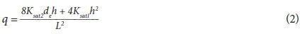
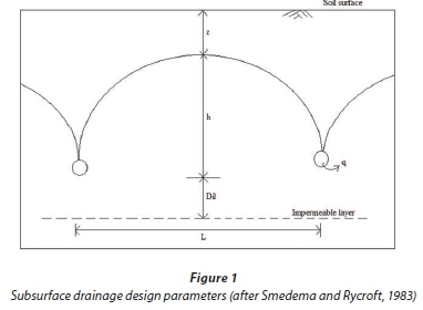
where: q is the drainage discharge (mm∙day^-1), L is the drain spacing (m); K_sat1 and K_sat2 are the saturated soil hydraulic conductivities (m∙day^-1) for soil layers above and below the drains, respectively; d_e is the equivalent depth (m); and h is the hydraulic head mid-way between two drains (m) (Oosterbaan, 1975; Fipps and Skaggs, 1989) (see Fig. 1). According to Oosterbaan (1975), d_e is a function of the depth to impermeable layer (Dil), drain depth, drain spacing and drain pipe radius.

 

 

The DRAINMOD model was chosen in this study because it has been tested under a wide range of climatic, crop and soil conditions. For instance, results of the DRAINMOD model performance, in Israel (Sanai and Jain, 2006), Iowa (Singh et al., 2006), South-eastern Purdue Agricultural Center (SEPAC), USA (Wang et al., 2006), Virginia, USA (Mc Mahon et al., (1988), Canada (Dayyani et al.,2009 and Schukla et al., 1994), Italy (Bixio and Bortolini, 1997), and North Carolina, USA (Skaggs 1982), confirm that the DRAINMOD model can reliably mimic subsurface drainage systems under a wide range of soil types and climatic conditions.

 

MATERIALS AND METHODS

Study site description

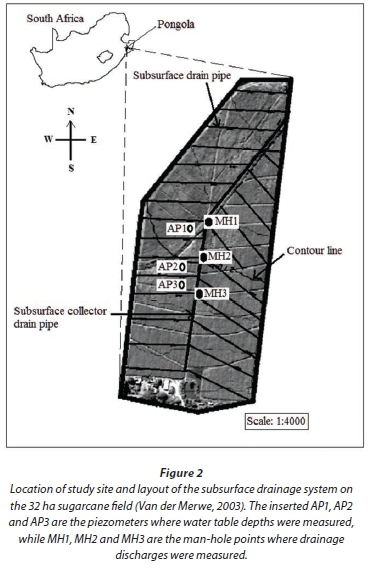
This study was conducted on a 32 ha sugarcane field in Pongola, KwaZulu-Natal Province, South Africa. The irrigation system adopted at the site is sprinkler irrigation with a design gross depth of irrigation at peak periods of 20 mm, irrigated after every 7 days. Pongola is located in the north-east of South Africa, close to the Swaziland border (Fig. 2).

 

 

The area is dominated by clay-loam and clay soils (Van der Merwe, 2003) with fairly gentle slopes. The Aridity Index (AI) for the area for the past 13 years is 0.12, indicating that the area is arid. Thus, from April to October (winter season), crop production is mainly through irrigation, while from November to March (summer season), crop production is dependent on both rainfall and irrigation.

The sugarcane field was first artificially drained, using an artificial subsurface drainage system in 1987. However, between 1995 and 2002, it was noticed that shallow groundwater tables were still affecting sugarcane growth. The subsurface drainage system was, therefore, abandoned and all the man-holes were filled up. This was followed by a recalculation of the drain depth and spacing, using the steady-state drain-spacing approach (Eq. 2) and the installation of the current subsurface drainage system in 2003. Details of the old and existing subsurface drainage systems are given in Table 1.

Field measurement of water table depths and drain discharges

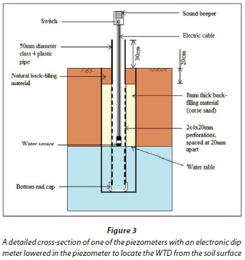
Water table depth data were obtained from piezometers, which were manually augured, using a 70-mm outside diameter auger to a depth of 1.7 m from the soil surface. A 50-mm internal diameter, class 4 PVC pipe with perforations was then lowered in each piezometer to a depth of 1.7 m, while ensuring that a 30-cm length was above the ground level to prevent runoff water from flowing in. End caps were fitted to both ends of the pipe to prevent the intrusion of materials into the piezometer. Coarse sand was backfilled throughout the whole perforated section of pipe (see Fig. 3). This was to prevent clogging of the perforations by clay and silt particles. Water table depths at each piezometer were measured by gradually lowering an electronic dip meter in the piezometer until a sound was heard. On the other hand, drainage discharges (q) in mm∙day^-1 were manually measured at 3 drainage outlet points (MH1, MH2 and MH3 in Fig. 2), using a bucket and a stop watch. It was quite difficult to find more drain outlet points where drain pipes were well-suspended, while at the same time providing enough clearance below them, so that a bucket could be accommodated to effectively measure the discharge.

 

 

For the first 3 weeks of the study (September 09 to 30, 2011), both DDs and WTDs were monitored every day, after which (October 01 to November 30, 2011) a monitoring frequency of once in 2 days was found to be appropriate. However, during the summer months of December 2011 to February 2012 the monitoring frequency was increased again to once per day due to frequent rainfall events.

Another WTD and DD data set for the October 1998 to September 1999 period was obtained from the Pongola Agricultural Office. According to Van der Merwe (2003), the methodology adopted in collecting the data was similar to the one described above.

Measurement of saturated soil hydraulic conductivity (K_sat)

Soil hydraulic conductivity (K_sat) values were measured using an in-situ method, i.e., the auger-hole method (Van Beers, 1983), which, according to Oosterbaan and Nijland (1994), is the most accurate and yet the simplest method, as opposed to laboratory methods. Prior to carrying out K_sat tests, 5 trenches were dug in the field (north, south, east, west and centre) to a depth of 2.3 m from the soil surface. This was done to characterize any heterogeneities in soil layer boundaries and to determine the number and thickness of the soil profile layers from the soil surface. The field was then divided into 3 sections (upper, middle and lower sections). Three 70-mm diameter auger-holes were drilled in each of the upper and middle sections, while 4 auger-holes were drilled in the lower section. This made a total of 10 auger-holes drilled in the whole field and used to determine a representative mean K_sat value to be used during model calibration, as recommended by Sobieraj et al. (2001).

The measurement procedure followed during the K_sat measurement is given by Van Beers (1983). It was observed that the auger smeared the surface of the auger-hole during the drilling process. The water level in the auger-hole was therefore left to stabilize for 1 day, in order to allow for a true water table to be established. On the following day, the water table depth in the auger-hole was determined and was followed by the bailing out of about 1 quarter of the water depth in the auger-hole, after which water level readings were taken every 10 s, using a Laser meter (HANNA Instruments) that was mounted on top of the access tube.

Weather data acquisition

Weather data (daily rainfall, potential evapotranspiration (PET) and minimum and maximum temperature) from 1998 to 2012 (14 years) was obtained from the Pongola SASRI weather station, located about 3 km from the study site (27° 24'S, 31° 35'E, and 308 m amsl). Weather data records for the years prior to 1998 were incomplete for some days; hence they could not be used because the DRAINMOD model requires completed daily weather data records. The DRAINMOD weather file also requires the inclusion of the irrigation component (mm∙day^-1) in the rainfall input file to account for any recharge to the soil system through irrigation. Hence, depths of irrigation water per irrigation day (mm∙day^-1) were measured using a rain gauge installed at the study site. This was followed by the modification of the rainfall file to include an irrigation component for each irrigation day throughout the whole study period. The PET, rainfall and temperature data files prepared in the Microsoft Excel spreadsheet were then converted to the DRAINMOD model data input format, using the DRAINMOD model weather data utility program.

DRAINMOD model calibration, evaluation and statistical analysis

Calibration is the process whereby default model input parameters are systematically adjusted to attain the best possible agreement between simulated and observed data sets, whereas validation is the process of testing the model's reliability in making appropriate predictions based on the calibrated parameters (Singh et al., 2006). In order to avoid ambiguities when making recommendations concerning the model's dependability, the October 1998 to September 1999 water table depth (WTD) and drainage discharge (DD) data were chosen to be used for calibration, while the data set from September 2011 to February 2012 was used for validation purposes. The adopted calibration procedure was similar to that of Dayyani et al. (2009) and Dayyani et al. (2010). Effective root zone depth for sugarcane was fixed at 60 cm from the soil surface (Savva and Frenken, 2002), and the growing period set from June to March.

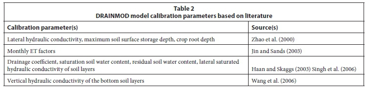
Literature indicates that the DRAINMOD model can be calibrated on a trial-and-error basis (Dayyani et al., 2010), by adjusting any or a set of input parameters presented in Table 2, until an optimal agreement between observed and simulated data sets is attained.

Time series of WTDs and DDs were simulated using the DRAINMOD model after every alteration of an input parameter or set of parameters. Simulated WTDs and DDs were then compared to observed WTDs and DDs. Initially, the agreement between the two data sets was assessed by visual judgments from WTD and DD hydrographs as proposed by Moraisi et al. (2007) and Dayyani et al. (2009). Later on 3 statistical parameters were used to characterize the DRAINMOD model performance, namely, mean absolute error (MAE) (Eq. 3) (El-Sadek, 2007), Pearson's product-moment correlation (R²) (Eq. 4) (Wang et al., 2006), also known as goodness-of-fit (Shahin et al., 1993; Legates and McCabe, 1999; Vazquez et al., 2002) and the coefficient of residual mass (CRM) (Eq. 5) (El-Sadek, 2007). These three statistical parameters were chosen because, according to Anderson and Woessner (1992) and Vazquez et al. (2002), they provide both quantitative and objective justifications in assessing the performance of a model in estimating a particular soil property.

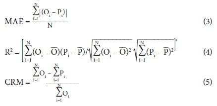
where: P_i is the simulated value, O_i is the observed value, and N is the number of data entries.

MAE describes the accuracy of a model in making correct predictions by measuring the average magnitude of errors between the simulated and observed values (Shahin et al., 1993; Legates and McCabe, 1999; Vazquez et al., 2002). According to Moraisi et al.(2007) and El-Sadek (2007), the MAE has a minimum value of 0.0, with values closer to 0.0 indicating a better agreement between measured and estimated values. The goodness-of-fit measures how the estimated and measured data sets correlate and has minimum and maximum values of 0.0 and 1.0, respectively, with values closer to 1.0 indicating a better correlation between the two data sets (Shahin et al., 1993; Legates and McCabe 1999; Vazquez et al., 2002). On the other hand, CRM characterizes the model's tendency to over-estimate (CRM<0) or under-estimate a property (CRM>0) (El-Sadek, 2007).

DRAINMOD simulation runs at various drain depths and spacing combinations

Scenarios were simulated to represent 2 soil types found at the study site, i.e., clay-loam and clay soil. The simulations were run for the September 2011 to February 2012 period. Input data for the simulations were those used in the model validation period. For clay soil, simulation scenarios were run with drain depths ranging from 1.4 to 1.8 m and drain spacing from 25 to 40 m at 3 m intervals. On the other hand, for clay-loam soil, simulation scenarios were run at drain depths ranging from 1.4 to 1.8 m, with drain spacing from 55 to 70 m. The selection of this drain depth and spacing simulation range for both soil types was based on a drain depth and spacing guide for KwaZulu-Natal developed by Russell and Van der Merwe (1997). For every simulation scenario, the mean WTD and DD were computed and were presented graphically.

 

RESULTS

Saturated hydraulic conductivities (K_sat)

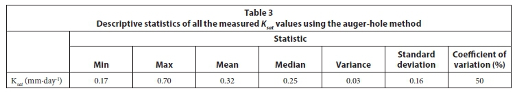
A summary of measured K_sat values for the bottom soil layer are shown in Table 3. The minimum and maximum K_sat values are 0.17 and 0.70 m∙day^-1, respectively, with a mean value of 0.32 m∙day^-1, and a standard deviation of 0.16 m∙day^-1. An analysis of the measured K_sat values shows that there is a high variability of K_sat values at the site with a coefficient of variation (CV) of 50%. Comparing the bottom layer K_sat values shown in Table 3 with top layer K_sat values, which according to Van der Merwe (2003) are in the range of 0.9 to 1.05 m∙day^-1, clearly shows that K_sat values for the top layer are higher than those for the bottom layer (0.17 to 0.70 m∙day^-1).

DRAINMOD model performance during calibration

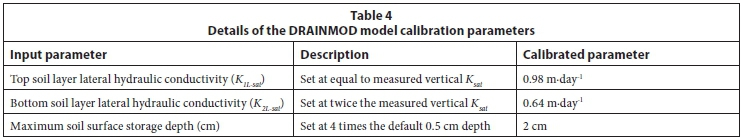
Details of the input parameters that were adjusted during the DRAINMOD model calibration and the extent to which the parameters were adjusted are shown in Table 4.

The lateral saturated hydraulic conductivity (K_2L-sat) for the bottom soil layer was set at twice the vertical saturated hydraulic conductivity (K_sat), while K_1L-sat for the top soil layer was set equal to the K_sat. It was assumed that the top soil layer K_sat values did not have significant changes during the 1998-2012 period. This was because the cropping system and cultivation practices at the site had not changed. Considering that crop residues were observed on the soil surface at the study site and that crop residues increase soil surface water storage (Gilley and Kottwitz, 1994), the soil surface water storage depth was set at 2 cm, contrary to the default 0.5 cm depth.

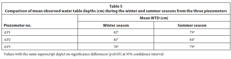
There were no significant differences among mean WTDs at piezometers AP1, AP2 and AP3, as can be seen in Table 5.

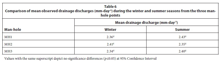
To avoid bias in selecting data to use in validating the DRAINMOD model, random numbers were assigned to AP1, AP2 and AP3. Water table depth data from AP2 were then randomly selected to be compared to simulated WTD data during validation. Similar to mean observed WTDs at the measured locations, there were no significance differences among mean DDs at MH1, MH2 and MH3 (see Table 6). Thus, DD data from MH2, which corresponded to AP2, were compared to simulated DDs.

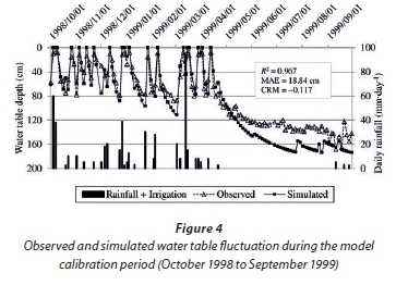
The results of time series of observed and simulated WTD and DD hydrographs during the calibration period are shown in Figs 4 and 5, respectively. As expected of arid and semi-arid climatic conditions, both observed and simulated WTDs show a fluctuating trend. Furthermore, it can be seen in Fig. 4 that fluctuation of WTD continued, even on rain-free and non-irrigation days, depicting the presence of unsteady state WTD and DD fluctuation. An analysis of the results in Fig. 4 further indicate that the model predicted shallow WTDs of less than 100 cm better than the deeper WTDs of more than 100 cm. In addition, the results show that generally the model predicted WTDs reasonably well, with a very strong R² value of 0.967 and a small MAE of 18.84 cm. A CRM of -0.117 indicates that the model has a general tendency of over-estimating WTDs.

 

 

 

 

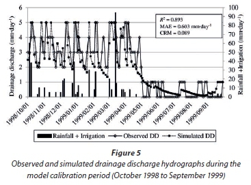
Results of time series observed and simulated DD hydrographs during the calibration period (September 1998 to October 1999) are shown in Fig. 5. Just like the DRAINMOD model calibration results in simulating WTDs, both the observed and simulated DD hydrographs show a fluctuating trend, depicting the presence of unsteady-state DD behaviour. A study of the results in Fig. 5 also show that the model predicted DDs of greater than 2 mm∙day^-1 better than DDs of less than 2 mm∙day^-1. Statistically, observed and simulated DD hydrographs show strong agreement, with a high R² and a small MEA of 0.893 and 0.603 mm∙day^-1, respectively.

A comparison of the R² values between pairs of observed and simulated WTD in Fig. 4 and DD in Fig. 5, shows that the model performed better in predicting WTD (R² = 0.967) than DD (R² = 0.893). Unlike the results of observed and simulated WTD (Fig. 4), in which the model over-estimated WTDs, contrary results were obtained in Fig. 5 (CRM>0), giving an indication that the model under-estimated DD during the calibration period.

DRAINMOD model performance during validation

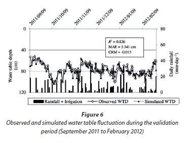
Results of the DRAINMOD model performance in simulating WTD during the validation period are shown in Fig. 6. A visual judgment of these results clearly shows that the observed and simulated WTD fluctuations correlated very well. This is statistically proven by a very strong R² value of 0.826 and a small MAE of 5.341 cm. The negative CRM value of -0.015 depicts that the model over-estimated WTD during the validation period. However, comparing the MAE of 18.84 cm obtained during the calibration period (Fig. 4) and the MAE of 5.341 cm obtained during the validation period, as seen in Fig. 6, gives an indication that there are smaller differences between individual pairs of observed and simulated WTD during the validation period than the calibration period.

 

 

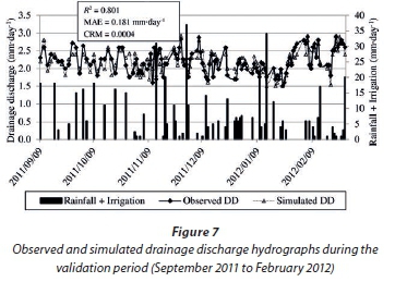
Results of the DRAINMOD model performance in predicting DDs during the validation period are shown in Fig. 7. A very good correlation between the observed and simulated drainage discharge hydrographs can visually be deduced from Fig. 7. Statistically, the correlation between the observed and simulated DDs is strong, with an R² value of 0.801 and a small MAE of 0.181 mm∙day^-1. Unlike the calibration results of observed and simulated DD (Fig. 5), where the model showed a general tendency of over-estimating WTDs, the results in Fig. 7 show that the DRAINMOD model has a general tendency of neither under-estimating nor over-estimating DDs, with a CRM of 0.0004, which is very close to zero.

 

 

Simulation scenarios at various drain depths and spacing combinations for two different soils types

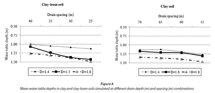
The calibrated DRAINMOD model was used to simulate WTDs and DDs for subsurface drainage systems installed in clay (K_sat = 0.24 m∙day^-1) and clay-loam soils (K_sat = 0.6 m∙day^-1).The results of mean simulated WTDs and their respective mean DDs at various combinations of drain depth and spacing are shown in Figs 8 and 9. It is evident that, when considering a constant drain depth, mean WTDs below the soil surface increase with decreasing drain spacing, and vice versa. For instance, in clay soil, it can be seen in Fig. 8 that for a subsurface drainage system installed at a drain depth of 1.4 m and its corresponding drain spacing of 40 m, the system establishes a mean WTD of 1.0 m. However, at the same 1.4 m drain depth, the system establishes a mean WTD of 1.11 m, when the drain pipes are installed at a closer spacing of 25 m.

Furthermore, the results in Fig. 8 show that, considering drain pipes installed in clay soil at drain depth ranging from 1.4 to 1.8 m, mean WTDs between 1.0 and 1.5 m can be established, when the drain pipes are installed at a spacing ranging from 25 to 40 m. On the other hand, by installing drain pipes at the same 1.4 to 1.8 m drain depth, mean WTDs between 1.0 and 1.5 m can be established in clay-loam soil when drains are installed at a relatively wider spacing, ranging from 55 to 70 m.

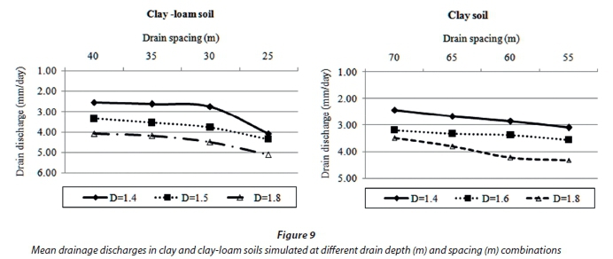
Results for mean DD, at various combinations of drain depth and spacing (Fig. 9), show that, when keeping the drain depth constant in both clay and clay-loam soils, mean DD rates increase with decreasing drain spacing and vice versa. Furthermore, it can be seen in Fig. 9 that, generally, mean DDs increase with increasing drain depth when drain spacing and type of soil are kept constant.

 

DISCUSSION

Performance evaluation of the DRAINMOD model

The model seemed not to simulate deep WTDs as accurately as was the case with shallow WTDs, particularly during the calibration period. The results were similar to those of the DRAINMOD model evaluation at a sugarcane field in north-eastern New South Wales, Australia, reported by Yang (2008), where the model also failed to simulate WTDs of more than 0.8 m as accurately as was the case with WTD less than 0.8 m. This was attributed to the model initially being developed to simulate WTDs and DDs under humid climatic conditions, where shallow water table depths are more prevalent (Sanai and Jain, 2006; Skaggs, 1978).

Nevertheless, the general performance results of the DRAINMOD model in simulating WTDs and DDs, during the calibration period, were better than the results reported by Dayyani et al. (2009) in Canada where they obtained R² values of 0.77 and 0.73, respectively. However, Dayyani et al. (2009) model validation results improved, with R² values of 0.93 and 0.90 for WTD and DD, respectively, which were higher than R² values found in this study. Dayyani et al. (2009) used very precise and automated water level and drainage discharge data loggers to locate the depth of the water table and measure daily drainage discharges, respectively. This could explain why model validation results reported by Dayyani et al. (2009) were better than the validation results found in this study.

The DRAINMOD model in this study predicted better WTDs than the results reported by Singh et al. (2006), who found R² values of 0.89 and 0.88 during the calibration and validation periods, respectively, which were very close to the R² values of 0.967 and 0.826 found in this study. The MAE of 5.41 cm found between observed and simulated WTDs during the validation period was smaller than the 7.0 cm found by Yang (2008).

Yang (2008) reports that the accurate estimation of K_sat values, to be used in the simulation of WTD and DD using the DRAINMOD model, enhances the adoptability of the model in an area, while the use of measured daily PET data improves the performance of the model. Notably, during their drainage simulation studies, both Singh et al. (2006) and Dayyani et al. (2009) used estimated PET data, soil water characteristics (SWC) and laboratory determined K_sat values as model inputs. The better performance of the DRAINMOD model in this study was to a large extent attributed to the use of measured PET data, soil water characteristics (SWC) and in-situ determined K_sat values as input parameters. In addition, the use of an electronic dip meter in locating the position of the WTD, as opposed to other methods, e.g., float meters, might have improved the quality of observed WTD data quite significantly. This reduced the differences between observed and simulated WTD values. Nonetheless, the use of WTD data loggers could have improved the quality of the results even more.

The slightly weaker agreement between the observed and estimated DDs in both the calibration and validation periods could be explained by the use of a low accuracy drainage discharge measurement method when measuring DDs, both during the 1998-1999 and 2011-2012 periods. The bucket and stop-watch method adopted in this study might have led to slightly less accurate measurements. Possibly, such errors resulted in greater differences between observed and simulated DDs. However, this could have been improved by using DD measurement equipment with a data-logging mechanism. Unfortunately, this could not be achieved because of resource constraints at the time of the study.

DRAINMOD simulation runs at varying drain depth and spacing combinations

Results of mean simulated WTDs and DDs confirmed the prevailing designs of installing drain pipes at shallow depths, in order to establish water WTDs near the soil surface and vice versa. The possible explanation for this water table behaviour could be reduced hydraulic heads at mid-drain spacing which, according to Dagan (1964), has a direct effect on both WTD at mid-drain spacing and drain discharge at drain outlet points.

However, considering a constant drain depth and soil type, and in as far as establishing deeper WTD is concerned, installing drain pipes at a closer spacing appeared to be a better option (Fig. 8). This was attributed to the elliptical water table shape with a very steep cone of depression, which, according to Rimidis and Dierickx (2003), increases the drain flux towards the drain pipe; hence the high water table drawdown (Δh) at mid-drain spacing and the increased drainage discharges.

On the other hand, the analysis of mean WTDs at various combinations of drain depth and spacing in clay and clay-loam soils in Fig. 8 suggested that closer drain spacing in clay soil and a wider drain spacing in clay-loam soils are more likely to establish the same mean seasonal WTD when drain depth is kept constant in both soil types. This was explained by differences in K_sat values for the two soil types, corroborating the description behind the Hooghoudt drain-spacing equation.

In a study of a similar nature conducted in the southern part of Louisiana, USA, Carter and Camp (1994) discovered that, by considering the same type of soil and a constant drain depth, shallow WTDs are established when drain pipes are installed at a wider spacing, while deeper WTDs are established when drain pipes are installed at a closer spacing. On the other hand, in southeast Queensland, Australia, Cook and Rassan (2002) found that considering a subsurface drainage system with drain pipes installed at the same drain depth in two soil types with different K_sat values, the same WTD can be established in both soil types, but with drain pipes installed at a wider spacing in the soil with a higher K_sat value, and vice versa. This indicates that the results found in this study corroborated well with study findings reported by Carter and Camp (1994) and Cook and Rassan (2002).

According to Oosterbaan (2002) and FAO (2007), the use of the Hooghoudt equation in arid and semi-arid conditions is based on a mean seasonal WTD and drainage discharge. Thus, it is apparent that under these climatic conditions the application of the Hooghoudt equation is not entirely based on a steady-state criterion, but a dynamic equilibrium of WTD and DD (Oosterbaan, 2002). It therefore follows that, based on the simulation results obtained in this study, respective drain depth, spacing and drainage discharge of 1.4 to 1.8 m, 55 to 70 m and 2.5 to 4.2 mm∙day^-1, would be appropriate to ensure safe WTD between 1.0 and 1.5 m depth for sugarcane grown in clay-loam soil. On the other hand, for sugarcane grown in clay soil, respective drain depth, spacing and drainage discharge of 1.4 to 1.8 m, 25 to 40 m and 2.5 to 5.1 mm∙day^-1, appeared to be appropriate to ensure a WTD between 1.0 m and 1.5 m from the soil surface.

It is recommended that the final selection of drain depth and spacing combination to be adopted at the site should be considered with caution, by making sure that drainage measures are not taken aggressively. Installation costs and available installation equipment in the area must be taken into consideration. In addition, efforts must also aim at selecting a drain depth and spacing combination that would considerably reduce irrigation water requirements by optimizing the soil moisture contribution to the root zone depth in the form of groundwater contribution.

 

CONCLUSIONS, RECOMMENDATIONS AND FUTURE RESEARCH

In this study, the reliability of the DRAINMOD model to predict WTD and DD was investigated at a sugarcane field in Pongola. Although the analysis of the DRAINMOD model evaluation results depicted that the model had a tendency of over-estimating WTDs (CRM<0) and under-estimating DDs (CRM>0), the general performance of the model in both the calibration and validation periods showed that it can still reliably be used as a subsurface drainage design tool under the Pongola conditions (R²>0.80). A detailed analysis of simulated WTDs and DDs at various drain depths and spacing combinations supported the generally prevailing design of installing drain pipes at a closer spacing in soils with low K_sat values and a wider drain spacing in soils of high K_sat values, as reported by other authors (e.g., Manjunatha et al. (2004) and Ritzema and Schultz (2010)). It therefore follows that, in order to maintain WTD between 1.0 to 1.5 m below the soil surface, the drain pipes in clay-loam soil be installed at a spacing of between 55 and 70 m, with a corresponding drain depth between 1.4 and 1.8 m and drainage design discharge in the range of 2.5 to 4.2 mm∙day^-1. For clay soil, simulated WTD and DD results revealed that WTD between 1.0 and 1.5 m can be achieved by installing drain pipes at a spacing of between 25 and 40 m, with a drain depth ranging from 1.4 to 1.80 m and corresponding drainage discharge ranging from 2.5 to 5.1 mm∙day^-1. Nevertheless, future verification of these drainage design criteria is of paramount importance before they can be widely adopted in the area. In addition, like previous DRAINMOD model simulation studies, long simulation periods are required to assess the control of shallow water tables in the area.

Most of the DRAINMOD model simulation runs in this study were made to suit the objectives of the study, which required WTD and DD simulated at various drain depth and spacing combinations only. However, the DRAINMOD model can also simulate the effects of varying drain depth and spacing on crop yields and drain effluent quality (e.g. Singh et al., 2006). It would therefore be interesting to test the reliability of the DRAINMOD model in simulating all of the abovementioned outputs. This will enhance the appropriate selection of drain depth and spacing combinations, not only based on WTD, but also on crop yields. Furthermore, this will also support future research linking the DRAINMOD model outputs (yield, water table depth, drainage discharge and effluent quality at various drain depth and spacing combinations) to a drainage system cost minimization model.

 

ACKNOWLEDGEMENTS

This research formed part of a Water Research Commission (WRC) Project (Project K5/2026//14) titled 'Development of Technical and Financial Norms and Standards for Drainage of Irrigated Agriculture'. We therefore thank the WRC for funding this research and all the individuals who formed the project team, for their guidance and assistance. We are particularly grateful to Mr Johan van der Merwe and Mr Sfundo Nkomo of the Pongola agricultural office for all the assistance they gave us during field work. Special thanks go to Prof Kourosh Mohammadi of Tarbiat Modares University, Iran, for his assistance in converting weather data files to the appropriate DRAINMOD format.

 

REFERENCES

ANDERSON MP and WOESSNER WW (1992) Applied Groundwater Modeling Simulation of Flow and Advective Transport. University Press, Cambridge. 296 pp.         [ Links ]

ASAE STANDARDS (1999) Standards Engineering Practices Data (46^th edn). American Society of Agricultural Engineering, St. Joseph, Michigan.         [ Links ]

BACKEBERG G (2000) Planning of research in the field of agricultural water management. Paper presented at an IPTRID workshop on 'Management of Irrigation and Drainage Research', 23-26 May 2000, Wallingford, Oxford. UK.         [ Links ]

BASTIAANSSEN WGM, ALLEN RG, DROOGERS P and STEDUTO P (2007) Twenty-five years modeling irrigated and drained soils: State of the art. Agric. Water Manage. 92 111-125.         [ Links ]

BIXIO V and BORTOLINI L (1997) Simulation of water flow in conventional and subsurface drainage with the DRAINMOD model. Irrig. Drain. 44 (2) 36-45.         [ Links ]

BOS MG and BOERS TM (2006) Land drainage: Why and how? In: Ritzema HP (ed.) Drainage Principles and Applications (3^rd edn). Alterra-ILRI, Wageningen University and Research Centre, Wageningen, The Netherlands. 23-32.         [ Links ]

CARTER CE and CAMP CR (1994) Drain spacing effects of water table control and cane sugar yields. Trans. ASAE 37 (5) 1509-1513.         [ Links ]

COOK FJ and RASSAN DW (2002) An analytical model for predicting water table dynamics during drainage and evaporation. J. Hydrol. 263 105-113.         [ Links ]

DAGAN G (1964) Spacing of drains by an approximate method. Irrig. Drain. Div. 90 (1) 41-56.         [ Links ]

DAYYANI S, MADRAMOOTOO CA, ENRIGHT P, SIMARD G, GULLAMUNDI A, PRASHER SO and MADANI A (2009) Field evaluation of DRAINMOD 5.1 under a cold climate: Simulation of daily mid span water table depths and drain outflows. J. Am. Water Resour. Assoc. 45 (3) 779-792.         [ Links ]

DAYYANI S, MADRAMOOTOO CA, PRASHER SO, MADANI A and ENRIGHT P (2010) Modeling water table depths, drain outflow, and nitrogen losses in a cold climate using DRAINMOD 5.1. Trans. ASAE 53 (2) 385-395.         [ Links ]

DWAF (2004) National Water Resource Strategy. Department of Water Affairs and Forestry, Pretoria, South Africa.         [ Links ]

EL-SADEK A (2007) Up-scaling field scale hydrology and water quality modeling to catchment scale. Water Resour. Manage. 21 149-169.         [ Links ]

FAO (2007) Guidelines and Computer Programs for the Planning and Design of Land Drainage. FAO Irrigation and Drainage Paper No. 62. Food and Agricultural Organization of the United Nations, Rome.         [ Links ]

FIPPS F and SKAGGS RW (1989) Influence of slope on subsurface drainage of hillsides. Water Resour. Res. 25 (7) 1717-1726.         [ Links ]

GILLEY JE and KOTTWITZ ER (1994) Maximum surface storage provided by crop residue. J. Irrig. Drain. Eng. 120 (2) 440-449.         [ Links ]

HAAN PK and SKAGGS RW (2003) Effect of parameter uncertainty on DRAINMOD predictions. Hydrology and yield. Trans. ASAE 46 (4) 1061-1067.         [ Links ]

HESS TM, LEEDS-HARRISON P and COUNSELL C (2000) WaSim Manual. Institute of Water and Environment, Cranfield University, Silsoe, UK.         [ Links ]

HOOGHOUDT SB (1940) General consideration of the problem of field drainage by parallel drains, ditches, watercourses, and channels. Publication No. 7 in the series 'Contribution to the knowledge of some physical parameters of the soil' (titles translated from Dutch). Bodemkundig Insitituut, Groningen, The Netherlands.         [ Links ]

HORTON R and KIRKHAM D (1999) Steady flow to drains and wells. In: Skaggs RW and Van Schilfgaarde J (eds) Agricultural Drainage. Agronomy Monograph No. 38. ASA/CSSA/SSSA, Madison, WI, USA.         [ Links ]

JIN CX and SANDS GR (2003) The long-term field-scale hydrology of subsurface drainage systems in a cold climate. Trans. ASAE 46 (4) 1011-1021.         [ Links ]

LEGATES DR and McCABE GJ (1999) Evaluating the use of 'goodness-of-fit' measures in hydrological and hydro-climatic model validation. Water Resour. Manag. 35 (1) 47-63.         [ Links ]

MANJUNATHA MV, OOSTERBAAN RJ, GUPTA SK, RAJKUMAR H and JANSEN H (2004) Performance of subsurface drains for reclaiming waterlogged saline lands under rolling topography in Tungabhadra irrigation project in India. Agric. Water Manag. 69 69-82.         [ Links ]

MCMAHON PC, MOSTAGHIMI S and WRIGHT SF (1988) Simulation of corn yield by a water management model for a coastal plain soil in Virginia. Trans. ASAE 31 (3) 734-742.         [ Links ]

MORAISI DN, ARNOLD JG, VAN LIEW MW, BINGNER RL, HARMEL RD and VEITH TL (2007) Model evaluation guidelines for systematic quantification of accuracy in watershed simulations. Trans. ASAE 50 (3) 885-900.         [ Links ]

OOSTERBAAN RJ (1975) Hooghoudt's Drainage Equation Adjusted for Entrance Resistance and Sloping Lands. International Institute for Land Reclamation and Improvement (ILRI), Wageningen, The Netherlands.         [ Links ]

OOSTERBAAN RJ and NIJLAND HJ (1994) Determination of saturated hydraulic conductivity. In: Ritzema HP (ed.) Drainage Principles and Applications. International Institute for Land Reclamation and Improvement (ILRI), Publication 16, Wageningen, The Netherlands.         [ Links ]

OOSTERBAAN RJ (2000) SALTMOD: Description of principles, user manual and examples of application. Special Report. International Institute for Land Reclamation and Improvement (ILRI), Wageningen, The Netherlands. http//:www.waterlog.info/saltmod.htm. 80pp.         [ Links ]

OOSTERBAAN RJ (2002) SALTMOD: Description of principles, user manual and examples of application. May 2002. International Institute for Land Reclamation and Improvement (ILRI), Wageningen, The Netherlands.         [ Links ]

RIMIDIS A and DIERICKX W (2003) Evaluation of subsurface drainage system performance in Lithuania. Agric. Water Manage. 59 15-31.         [ Links ]

RITZEMA HP and SCHULTZ B (2010) Optimizing subsurface drainage practices in irrigated agriculture in the semi-arid and arid regions: Experiences from Egypt, India and Pakistan. Irrig. Drain. DOI:10.1002/ird.585.         [ Links ]

ROMANO N and PALLADINO M (2002) Prediction of soil water retention using soil physical data and terrain attributes. J. Hydrol. 265 56-75.         [ Links ]

RUSSELL WB and VAN DER MERWE JM (1997) Subsurface drainage. In: KwaZulu-Natal Farmland Conservation. KwaZulu-Natal Department of Agriculture, Pietermaritzburg, South Africa.         [ Links ]

SANAI G and JAIN PK (2006) Evaluation of DRAINMOD in predicting water table heights in irrigated fields at the Jordan Valley. Agric. Water Manage. 79 137-159.         [ Links ]

SAVVA A and FRENKEN P (2002) Planning, Development and Evaluation of Irrigated Agriculture with Farmer Participation. FAO Sub-regional Office for East and Southern Africa, Harare, Zimbabwe.         [ Links ]

SCHUKLA MB, PRASHER SO, MADANI A and GUPTA GP (1994) Field validation of DRAINMOD in Atlantic Canada. Can. Agric. Eng. 36 (4) 205-213.         [ Links ]

SHAHIN M, VAN OORSCHOT HJL and De LANGE SJ (1993) Statistical Analysis in Water Resources Engineering. A.A. Balkema Publishers, Leiden, The Netherlands. 394 pp.         [ Links ]

SINGH R, HELMERS MJ and ZHIMING Qi (2006) Calibration and validation of DRAINMOD to design drainage systems for Iowa's tile landscapes. Agric. Water Manage. 85 221-232.         [ Links ]

SKAGGS RW (1976) Determination of hydraulic conductivity-drainable porosity ratio from water table measurements. Trans. ASAE 19 (84) 73-80.         [ Links ]

SKAGGS RW (1978) A water management model for shallow water table soils. Technical Report No. 134. Water Resources Research Institute, University of North Carolina, Raleigh, NC, USA.         [ Links ]

SKAGGS RW (1980) Methods for design and evaluation of drainage water management systems for soils with high water tables, DRAINMOD. North Carolina State University, Raleigh, NC, USA.         [ Links ]

SKAGGS RW (1982) Field evaluation of a water management simulation model. Trans. ASAE 25 (4) 666-674.         [ Links ]

SMEDEMA LK and OCHS WJ (1998) Needs and prospects for improved drainage in developing countries. Irrig. Drain. Syst. 12 359-369.         [ Links ]

SMEDEMA LK and RYCROFT DW (1983) Land Drainage Planning and Design Systems. Cornell University Press, Ithaca, NY, USA.         [ Links ]

SOBIERAJ JA, ELSENBEER H and VERTESSY RA (2001) Pedotransfer functions for estimating saturated hydraulic conductivity: implications for modeling storm flow generations. J. Hydrol. 251 202-220.         [ Links ]

VAN BEERS WFJ (1983) The auger hole method: A field measurement of the hydraulic conductivity of soil below the water table. International Institute for Land Reclamation and Improvement (ILRI), Wageningen, The Netherlands.         [ Links ]

VAN DER MERWE JM (2003) Subsurface drainage design. Department of Agriculture and Environmental Affairs, Pongola, KwaZulu-Natal.         [ Links ]

VANDERSYPEN K, KEITA ACT, COULIBALY B, RAES D and JAMIN JY (2007) Drainage problems in the rice schemes of the office du Niger (Mali) in relation to water management. Agric. Water Manage. 89 153-160.         [ Links ]

VAZQUEZ RF, FEYEN L, FEYEN J and REFSGAARD JC (2002) Effect of grid-size on effective parameters and model performance of the MIKE SHE code applied to a medium sized catchment. Hydrol. Process. 16 (2) 355-372.         [ Links ]

WANG X, MOSLEY CT, FRENKENBERGER JR and KLADIVKO EJ (2006) Subsurface drain flow and crop yield predictions for different drain spacing using DRAINMOD. Agric. Water Manage. 79 113-136.         [ Links ]

YANG X (2008) Evaluation and application of DRAINMOD in an Australian sugarcane field. Agric. Water Manage. 95 439-446.         [ Links ]

ZHAO SL, GUPA SC, HUGGINS DR and MONCRIEF JF (2000) Predicting subsurface drainage, corn yield, and nitrate nitrogen losses with DRAINMOD-N. Environ. Qual. 29 (3) 817-827.         [ Links ]

 

 

Received 18 December 2013
Accepted in revised form 3 March 2015

 

 

* To whom all correspondence should be addressed. ☎ +27 (33) 260-6064; Fax: +27 (33) 260-5818; e-mail: senzanjea@ukzn.ac.za