


Services on Demand
Article
 English (pdf)
 Article in xml format
 Article references
Indicators

Related links
-
 Cited by Google
 -
 Similars in Google
Share

 Permalink
Water SA
On-line version ISSN 1816-7950
Print version ISSN 0378-4738
Water SA vol.40 n.3 Pretoria Jun. 2014
http://dx.doi.org/10.4314/wsa.v40i3.11
Downstream flow top width prediction in a river system
Parthasarathi Choudhury; Nazrin Ullah*
Department of Civil Engineering, NIT Silchar, Assam, India, PIN: 788010
ABSTRACT
ANFIS, ARIMA and Hybrid Multiple Inflows Muskingum models (HMIM) were applied to simulate and forecast downstream discharge and flow top widths in a river system. The ANFIS model works on a set of linguistic rules while the ARIMA model uses a set of past values to predict the next value in a time series. The HMIM model assumes a power-law relationship between water discharge and flow top width at a section. The models were used to simulate and forecast discharge and flow top width at a downstream section in the Barak River system in India. Flow top widths corresponding to different flow depths at the downstream section were estimated using a digital elevation model (DEM). The parameters in the hybrid model were estimated by applying Non-dominated Sorting Genetic Algorithm II (NSGA-II). The study shows that the power-law relationship involving section characteristics can describe the top width versus discharge relationship for a section. The models allow direct estimation of the downstream flow top width on the basis of upstream flow variables. Results obtained in the study show that performances of the HMIM, ANFIS and ARIMA models are satisfactory, having average prediction errors of less than 7% of the average value of the observed series. Application of the ANFIS, ARIMA and the HMIM models to the studied river system demonstrate the suitability of the models in simulating and forecasting downstream flow top width in river systems.
Keywords: River system, flow top width, genetic algorithm, flood flow, hybrid model
INTRODUCTION
River flood forecasting and warning is one of the most important components of flood management. Reliable forecasts of future river flow conditions and early warning is necessary to take preventive measures and to mitigate flood damage. In addition to depth of flow and discharge, flow top width, which represents the extent of inundation, is an important factor for assessing the impact of flooding. Estimation of the flow top width at a channel section is important to get an idea of the impact and probability of flooding. Until recently, different types of models have been used for simulating fluvial flows in general and flood inundation in particular. These can range in complexity from using high resolution digital elevation models (DEM) capable of giving the flooded area (Zheng et al., 2008) to the use of full three-dimensional solutions of the Navier-Stokes equations (Yu and Lane, 2006; Gilles, 2010). Pappenberger et al. (2006) used the St. Venant equations for flood inundation prediction and applied Generalised Likelihood Uncertainty Estimation (GLUE) methodology to account for the uncertainty in forecasting inundation. Hashmi et al. (2012) used Mike 11 software to develop a rainfall-runoff model for Lai Stream Basin, Pakistan, and simultaneously generated flood maps for the area. Two-dimensional finite difference and finite element models (Anderson and Bates, 2000) have also been used to analyse flood movement in river reaches. Though the two-dimensional models give better representation of flood flow and flood inundation, these require extensive physical data and computational efforts for model calibration. Acquiring the required physical data for river reaches is often difficult; the non-availability of a pertinent dataset is a drawback that usually restricts model development and its applications.
Apart from the abovementioned models, extensive use of data-driven models, time- series models and lumped empirical Muskingum models in flood flow modelling can be found in the literature. Data-driven models such as the adaptive neuro-fuzzy inference system (ANFIS), artificial neural network (ANN) and fuzzy logic (FL) have been found to be potentially useful in modelling time-series problems. The main advantage of these models is that they do not require specifying a functional relationship a priori; instead they self-organise the structure; adapt to it in an interactive manner, and can learn the underlying relationship(s) from the input-output data sets. In the hydrological forecasting context, application of data-driven models can be found in the works of Liong et al.(2000), Bazartseren et al. (2003), Chen et al. (2006), Jacquin and Shamseldin (2006), and Dastorani et al. (2009), among others. Fernandez et al. (2010) applied a neuro-fuzzy model for level prediction in Magdalena River, Columbia, and reported better performance by the ANFIS model compared to the deterministic models. The ANFIS model works on a set of linguistic rules and can handle imprecision and uncertainty inherent in the model and the data structure. Studies which have reported on the applications of ANFIS reveal that the model is useful in simulating and forecasting hydrologic time series.
As hydrologic events are essentially time-dependent, a number of time-series models have been used in modelling the problems. Time-series models such as Autoregressive Integrated Moving Average (ARIMA), and Autoregressive Moving Average (ARMA) models have been proposed and have been widely used for modelling hydrological time series (Box and Jenkins, 1976; Wang et al., 2006; Martins et al., 2011). An ARIMA model is a generalisation of an ARMA model; it makes time-series stationary in both calibration and forecasting phases. Khashei and Bijari (2010) applied hybrid ANN-ARIMA models for forecasting time series, obtaining improved model performances. A recent investigation that evaluates performances of ARIMA and ARMA models in forecasting river flow is reported by Valipour et al. (2012). There is a considerable volume of literature on the applications of ARIMA and ARMA models in forecasting hydrologic time series. Extensive application of these models in hydrology is mainly due to the fact that these models have the capability of generating new sequences of time-series having the same statistical parameters as the observed series.
Another model that is widely used by researchers in modelling flood movement in river reaches is the Muskingum model (McCarthy, 1937). The model is a lumped empirical model and is based on storage-continuity relationships. The basic Muskingum model is applicable to a single river reach (Gasiorowski, 2009; Balaz et al., 2010) and allows for estimating and forecasting downstream flow rates on the basis of upstream flows. Some recent applications of the Muskingum model can be found in the works of Ilaboya et al. (2011) and Kumar (2011). O'Donnell (1985) and Khan (1993) modified the basic Muskingum model to apply it to a river system. For a river system the model can be written using the equivalent inflow concept (Choudhury et al., 2002, 2007); the equivalent inflow model is useful in estimating and forecasting common downstream outflow on the basis of several upstream flows.
In the case of river flow, a power-law relationship involving sectional characteristics is used to estimate the discharge at a section. The Y-Q model assumes discharge to be a function of depth of flow and sectional characteristics; parameters in the model representing section characteristics are estimated using depth-discharge data for a section. Top width of flow may be considered as a function of flow depth for sections having profiles that can be described by using standard curves or a combination of standard curves. Power models applicable to the relationship between depth and discharge may also be suitable for describing the top width-discharge (T-Q) relationship for sections having linear and power relationships between depth and top width (Bjerklie, 2005; Yang et al., 2013). A single rating curve described by a power-law may be adequate if the flow depth is less than the bank-full depth; however, if it exceeds the bank-full depth a single rating curve may not give good results as roughness and other flow conditions would vary significantly. In that case, a compound rating curve (Jain, 2008), having different segments in the compound curve which are described by different power-law or other equations, may be used to enhance model performance. Discharge for a section defined in terms of the top width variable, and as given by the (T-Q) model, is useful in reformulating the flow models in terms of the top width variable. In the case of the Muskingum model, a nonlinear hybrid model form can be obtained if the downstream discharge is substituted by the estimate obtained using the flow top width variable. The hybrid model relates downstream flow top width with the upstream flow rates and allows direct estimation and forecasting of downstream flow top width in a river reach.
In the present study, HMIM, ANFIS and ARIMA models incorporating discharge and flow top width variables are applied to forecast and/or simulate outflow and flow top width at a downstream station in a river system in India. Flow top width corresponding to different flow depths at the downstream section is estimated using DEM. The HMIM model assumes a power-law relationship between water discharge and flow top width at a section. Parameters in the HMIM model are estimated by applying Non-dominated Sorting Genetic Algorithm II (NSGA-II). Model applications show that the estimated parameter set, when used in the multiple inflows Muskingum (MIM) model and in the HMIM model, result in downstream discharge and flow top width predicted values that closely match the observed data. HMIM, ANFIS and ARIMA models allow direct estimation of the downstream flow top width on the basis of upstream flow variables, extending the applicability of the models to simulate/forecast flow top width in a river system. Model capabilities for simulating and forecasting flow top width are important and useful for assessing the probability and impact of flooding at a river section.
MODELS
The Muskingum model for a river system having a number of upstream flows and a common downstream outflow can be written as (Choudhury, 2007):
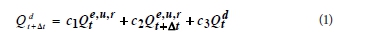
where:
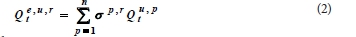
where:
Qte.u.r = equivalent flow at a point r in the basin for n upstream flows measured at different locations
Qt-u,p = flow at an upstream point p
σ p,r = shift factor associated with the transfer of upstream flow from p to r
Qtd = outflow at the common downstream station in the river system
c1, c2 and c3 are the routing coefficients for time interval Δt
The model given in Eq. (1) can be rewritten in terms of the Muskingum model parameters k and x using the relationships, c1= (Δt+2kx)/[Δt+2k (1-x)]; c2= (Δt-2kx)/[Δt+2k(1-x)]and c3= [-Δt+2k (1-x)]/ [Δt+2k (1-x)].
In the case of river flow, discharge passing through a section can be modelled using section characteristics and the depth of flow. For a section the discharge, Qt (*) is usually estimated from the measured depth of flow, Yt(*) employing a power-law (Y-Q) relationship. The Y-Q model describes the depth-discharge relationship satisfactorily and is regarded as an established model. As determined by the shape characteristics , top width at a section is a function of depth of flow, and, on the basis of the functional relationship existing between top width and depth of flow, an independent relationship between top width, Tt(*) and discharge, Qt (*) for a section can be defined. The T-Q model relies on the Y-T relationship at a section, and, depending on the shape factor, different types of model may be suitable for defining top width-discharge relationships for a section; the power-law model is an appropriate model if the depth-top width relationship for a section follows a power law. For such river sections the T-Q model written in terms of sectional properties may be given as:
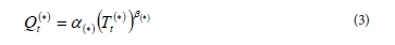
where:
The symbol (*) indicates a section
Qt (*) = instantaneous water discharge (m3/s) at a section (*) at time t
α (*), β(*) = rating curve parameters reflecting water discharge characteristics at a section
Tt(*) = instantaneous flow top width at a section at time t.
The T-Q model given in Eq. (3) is single valued, describing a one-to-one correspondence between water discharge and flow top width variable at a section. Further consideration shows that Eq. (3) is in agreement with the Y-Q model applicable to a river section. As defined by the sectional properties and on the basis of flow top width, Tt(*), Eq. (3) provides an estimate for the water discharge, Qt(*) passing through a section; the estimate for the water discharge may be used to reformulate flow models incorporating a flow top width variable for a section.
Equation (1) gives the multiple inflows Muskingum model applicable to a river system. The model can be calibrated using discharge values for various upstream and downstream stations . As given in Eq. (2), the equivalent inflow for a river system is a function of upstream flows, Qtu,p, and shift parameters , σpr given by Qte,u,r=f(σpr, Qu,p). Referring to Eq. (3), the term Qte,u,,r in Eq. (2) can be expressed as a function of upstream top widths, Ttp, upstream section properties αp, βp, and the shift parameters σp,r,  , p = 1,2,3.. n. Using the estimate for water discharge given by Eq. (3) and employing the functional relationship between equivalent inflow and upstream flow top widths, Qe,u,r = g(αp, βρ, σp,r, Ttp)in Eq. (1), the Muskingum model for a river system can be rewritten in terms of flow top width variables only. If the estimate for water discharge as defined by Eq. (3) is used to substitute the downstream discharge only, a hybrid Muskingum (HMIM) model for the river system, as given in Eq. (4), can be obtained.
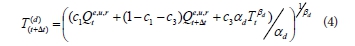
Using water discharge for different upstream stations, Eq. (4) may be expanded and written as follows:
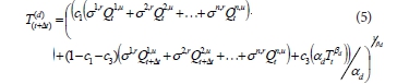
Here:
T(*)(d) denotes downstream flow top width
t, t+Δt represents the time-period
c1, c2, c3 are the routing coefficients.
Equation (5) gives the HMIM model incorporating discharge and flow top width variables for a river system. The model is highly non-linear involving a number of parameters. The model relates discharges separated by a time interval At for various upstream and downstream stations in a river system, satisfying continuity requirements adhering to the Muskingum principle of flow movement in river reaches. The model allows for directly estimating downstream flow top width on the basis of water discharges for different upstream stations.
Model parameters in Eq. (5) could be estimated by minimising the difference between the observed and computed downstream flow top width values. Εquation (5) being the hybrid form of the Muskingum mo del given by Eq. (1), a parameter set for a river system may be identified to best satisfy both models. Eq. (1) and Eq. (5) may also be written in terms of parameters k and x to estimate the parameters describing river reach characteristics. To estimate optimal parameters satisfying the Multiple Inflows Muskingum (MIM) model and the HMIM model, objective functions framed using Eq. (1) and Eq. (5) may be considered. The HMIM model given by Eq. (5) is highly nonlinear, involving a number of parameters; calibration of the model using gradient-based techniques may be difficult due to computational problems. Population-based search techniques using genetic algorithms (GA) have the capability of optimising non-linear functions efficiently. The technique gives a number of alternative solutions along with the best parameter set values for a problem. The objective functions given in Eq. (6) and Eq. (7) that represent minimisation of the sum of the squared differences between observed and computed downstream values may be used to estimate the model parameter set for a river system. With estimated parameter values, Eq. (1) and Eq. (5) may be used to simulate downstream discharge and flow top width in a river system on the basis of water discharges at several upstream stations.
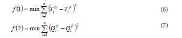
where:
T0, QO represent observed flow top width and observed discharge, while
TP, QP represent the predicted flow top width and predicted water discharge at the downstream station, respectively
Minimisation of the objective functions given by Eqs. (6) and (7) leads to estimated model parameters c1, c3/k, x and σρr, ad, βά for a river reach. The estimated parameters may be used to develop downstream flow top width simulation and forecasting models for a river system. Model calibration applying the genetic algorithm technique may be performed using a multi-objective optimisation routine. NSGA is a multi-objective evolutionary algorithm that starts with an initial population which is progressively improved through iteration leading to a number οf feasible solutions. The optimisation technique is based on natual selection and the mechanisms of population genetics, i.e., the biological process of survival and adaptation. NSGA-II is an improved version of NSGA (Srinivas and Deb, 1994) and can optimise multiple objectives. The algorithm uses a fast non-dominating sorting approach to discriminate solutions on the basis of Pareto dominance and optimality.
Forecasting models
The forecasting form for the flow top width simulation model given by Eq. (5) can be defined for a time step, Δt' = 2kx. For Δt' = 2kx, C/2 = 0 and the forecasting form for discharge and top width simulation models that provide downstream values estimated Δt' = 2kx time periods ahead can be obtained as:
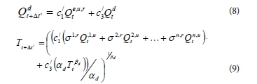
For a river reach with estimated Muskingum model parameters k, x/c1,c3; shift parameter σp,r, and the rating parameters αd,βd for the downstream section, Eqs. (8) and (9) can be defined and used to obtain downstream water discharge and flow top width estimated Δt' time units ahead.
ANFIS model
ANFIS is an artificial intelligence technique that has been successfully used for mapping input-output relationships based on available data sets (Jang et al., 1993; Bisht and Jangid, 2011). ANFIS is based on the first-order Sugeno-fuzzy inference system proposed by Jang (1993), and uses neural network learning algorithms and fuzzy reasoning to map an input space to an output space. With the ability to combine the numeric power of a neural system with the verbal power of a fuzzy system, ANFIS has been found to be powerful in modelling numerous processes. The model works on a set of linguistic rules developed using expert knowledge. The fuzzy rule base of the ANFIS model is set up by combining all categories of variables. For example, if there are n inputs and if each input is divided into c categories then there will be cn rules. For 3 inputs, x, y and z, and each input having 3 categories, viz., low, medium and high, there would be 27 rules in the rule base; the output for each rule is written as a linear combination of input variables and a constant term. A typical rule that gives the output when all three inputs are in category 'low' may be written as:
Rule 1: If x is low, y is low and z is low then the output is:

Similarly, outputs for all possible rules are taken as linear combinations of input variables and a constant term. The coefficients a(...); b(...); c(...); d(...) are parameters of the output functions and these parameters are determined through training.
For each of the rules triggered, memberships of the input variables x, y, z are computed through learning. The result of T-norm gives the weight to be assigned to the corresponding output. Finally, outputs from all triggered rules are combined to give a single weighted average output given by:
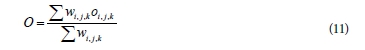
Here, i, j, k are the input categories.
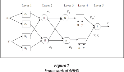
In order to develop a fuzzy inference model, the parameters defining the shape of the membership functions are identified by the back-propagation learning algorithm, whereas the parameters in the output function a(.); b(.); c(.); d(.) are determined by the least-square type method. The model possesses features of both neural networks and fuzzy control systems, such as learning abilities, optimisation abilities and human-like 'if-then' rule thinking. The framework of ANFIS is shown in Fig.1. The model can efficiently map multiple inputs to a single output and may be used to simulate and forecast downstream flow rates and flow top width in a river system receiving inflows at several upstream locations.
ARIMA model
The ARIMA model is a general time-series model for forecasting popularised by Box and Jenkins (1976). The ARIMA model is fitted to time-series data to better understand the data and to predict future points in the series. It uses 3 components for modelling the serial correlation in the time-series data. The first component is the autoregressive term (AR), the second component is the integration (I) order term. Each integration order corresponds to differencing the time series. I(d) represents differencing the data 'd' times and the third component is the moving average (MA) term. The general form of the ARIMA model (l, d and q) is given by:
where:
i = 1,2,3..J and j=1,2,3....q.
yt is a stationary stochastic process and has a non-zero average
a0 is a constant coefficient
ai represents the autoregressive coefficient
bj represents the moving average coefficient ej is the white noise disturbance term.
In evaluating the performance of an ARIMA model, Bayesian Information Criterion (BIC) and Akaike Information Criterion (AIC) values may be used to determine if an ARIMA model with a specific set of l, d and q parameters is a good statistical fit. The AIC value gives the degree of information lost due to model fitting. For a given data set, a number of candidate models having different l, d and q parameters may be fitted and the model giving lowest values for AIC and BIC can be selected as the best model.
STUDY AREA AND DATA SET
The hybrid Muskingum model, ANFIS and ARIMA models were applied to a river network in Barak Basin in India. The Barak River is the second-largest river in the north-eastern region of India and rises in the state of Nagaland at an elevation of approximately 2 300 m amsl. The drainage area of the river is approx. 14 500 km2. The Barak valley has a population of about 2.98 million. The sub-basin is situated on the route of the southwest monsoon; it receives an annual rainfall of 2 500 to 4 000 mm with 80-85% of the annual rainfall occurring from mid-April to mid-October. The problem of flooding is very complex and acute in the valley. Almost every year during the monsoon the valley receives 2-3 flood waves, inundating a vast part of the valley and causing widespread damage. With agriculture being the main occupation of about 70-75% of the population in the valley, the problem of recurrent flooding jeopardises economic growth and development in the region.
In this study, a river network bounded by 3 upstream inflow gauging stations and a downstream outflow gauging station in the mainstem of the Barak River was selected for application of the models. Details of the study area along with the river system are shown in Fig. 2.
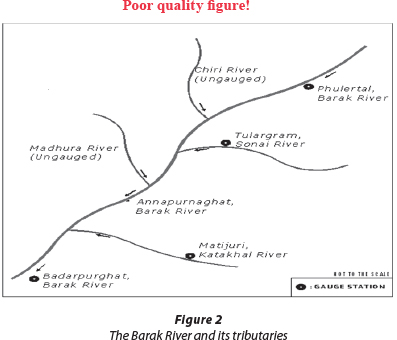
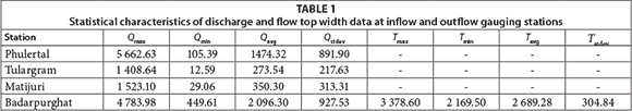
The upstream gauging stations are located at Phulertal in the main river Barak, Tulargram in the tributary Sonai and at Matijuri in the tributary Katakhal. There are also some minor ungauged tributaries that join the reach between Phulertal and Badarpurghat. As flow data for these tributaries are not available, only flows from the major upstream gauged catchments were used to simulate downstream flows and flow top width in the river system. It may be noted that inclusion of two additional tributary flows increases model agreement with the continuity relationship, compared to the basic Muskingum model in which only the upstream main channel flow is used. Applying the models, downstream flow top width is estimated/ forecast using upstream flow rates. Hourly discharge and stage data for all four gauging stations were obtained from the Central Water Commission (CWC), Shillong. In order to calculate the flow top width for the downstream station, toposheets at a scale of 1:50 000 obtained from Survey of India were used, and were scanned and digitised. Using ArcGIS, a DEM depicting surface elevations for the downstream locations in the river system was prepared. Corresponding to a recorded flow depth at the downstream station, the width of the water surface across the stream, depicting the flow top width, was measured. A total of 241 datasets containing upstream discharges and downstream discharge/flow top width data for the selected river system were used in this study. Out of the 241 datasets, the first 50% of each dataset was used for training and the remaining data was used for testing (25%) and calibration (25%). The statistical characteristics, maximum, minimum, average and standard deviation, for the observed discharge series at upstream gauging stations Phulertal, Tulargram and Matijuri, and for discharge and top width series at the downstream gauging station Badarpurghat, are summarised in Table 1.
APPLICATIONS
Applicability of the hybrid multiple inflows Muskingum model, ANFIS and ARIMA models in simulating and forecasting water discharge and flow top width for a downstream section is demonstrated for a river network in Barak Basin, India.
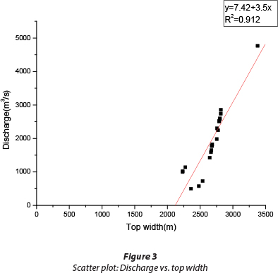
Discharge and flow top width simulation models for the river system represented by Eqs. (1) and (5) were calibrated using 241 pairs of inflow, outflow and common downstream flow top width data for the river system. Water discharge data for 4 gauging stations in the river system were obtained from CWC, Shillong. Observed flow top width data for the downstream station were obtained using DEM and applying the ArcGIS tool. The hybrid model incorporating water discharge and flow top width variables was used to obtain simulated and 2 hours ahead forecasted discharge and flow top width at a downstream section in the river system. To determine flow top widths at the downstream section corresponding to a set of recorded flow depths in the river system, flow top width across the downstream section was measured using the DEM. Correlation coefficients between flow top width and discharge, and flow top width and depth of flow, at the downstream station were found to be 0.965 and 0.935, respectively. The correlation coefficient values show that top width of flow has a relationship with discharge and depth of flow at the section. Figure 3 shows a scatter plot of discharge vs. flow top width at the downstream section, Badarpurghat. The scatter plot (R2=0.912) also indicates the existence of a functional relationship between flow top-width and the discharge passing through the section.
Concurrent water discharges observed at 3 upstream stations and the corresponding flow top width measured for the downstream station were used in Eq. (5) to develop the HMIM model. Water discharge and flow top width data measured at 1-h intervals were used in the study; two objective functions written using Eq. (1) and Eq. (5) were used to estimate the parameters. NSGA-II was used to minimise the objective functions representing the sum of the squared deviations between downstream observed and computed values, obtaining estimates for the unknown parameters k, x,σprand αd,βd. Estimated parameters were used in the MIM model and HMIM model given by Eq. (1) and (5), respectively, to obtain simulated downstream water discharge and flow top width values for the reach. The estimated parameter values are listed in Table 2. Equation (1) gives multiple inflow Muskingum model formulation for a river system, replacing a river network by an ordinary Muskingum reach, and satisfies the continuity requirements in a relative sense (Choudhury, 2007). In the present model formulation, the continuity requirement is also satisfied in a relative term as the model selects a downstream hydro graph given by the parameters ad, βd and an upstream hydrograph defined by the parameters σpr to estimate the Muskingum model parameters k, x for the reach. To estimate model parameters using downstream flow variations as close as possible to the actual variation, a third objective function framed applying Eq. (3) may be used. Performance of the models was evaluated using standard statistical criteria, the coefficient of correlation (CORR), Nash-Sutcliffe model efficiency coefficient (CE), root mean square error (RMSE) and mean absolute error (MAE). The coefficient of correlation describes how the two data sets move; when CORR=1 this indicates perfect positive linear correlation between the predicted and observed series and the two data sets move in the same direction. Coefficient of efficiency (CE) is an important statistic describing model fitness. A value of CE=1 indicates a perfect model fit while CE=0 indicates that the model is as good as the mean model, whereas RMSE indicates the absolute fit of the model to the data, i.e., how close the observed data points are to the model's predicted values. On the other hand, MAE measures the average magnitude of the errors in a set of forecasts, without considering their direction. Performances of HMIM and MIM models in simulating downstream flow top width and discharge are listed in Table 2.
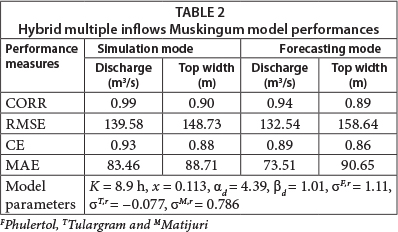
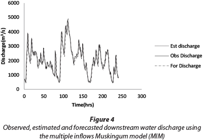
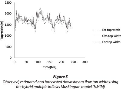
The estimated model parameters k and x are used to compute the forecasting model coefficients c'1 and c'2 for the river system. The forecasting lead time for the MIM and HMIM models is computed to be At'=2.01 h and the forecasting model coefficient values are computed to be c1' = 0.119 and c3' = 0.881. The models are used with present flow rates at the upstream stations and present flow rate/top width values for the downstream station, obtaining forecasts for the downstream possible discharge rates/flow top width values 2 hours ahead. The forecasting model performances for the river system are also listed in Table 2. Results given in Table 2 show that CE values for MIM and HMIM simulation and forecasting models are more than 0.85 and indicate satisfactory performances. The CE values for simulating downstream water discharge on the basis of upstream water discharges are close to 1; CE values obtained for simulating downstream flow top width on the basis of upstream flow rates are more than 0.85. Simulated and forecast downstream water discharge and flow top widths for the river system are given in Figs 4 and 5. The flow top width value is usually required for estimating the expanse of flow at a section; the HMIM model equipped with forecasting capabilities can provide downstream flow top width values estimated/forecast on the basis of upstream flow rates. Model capabilities in forecasting downstream flow top width values are important as such advance information is beneficial for taking precautionary measures against flood damage and for mitigating flood losses.
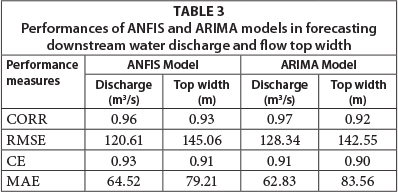
The two other models, ANFIS and ARIMA, were also used to forecast the discharge and flow top width at the downstream station 1 hour ahead. The ANFIS model was selected by conducting trials using different input categories, types of membership functions and the training algorithm. The ANFIS model with triangular membership functions for 3 input categories and constant output membership functions was selected on the basis of minimum RMSE. The selected ANFIS model has 4 inputs representing concurrent flows at 3 upstream and 1 downstream location; each of the 4 inputs has 3 categories giving 81 rules. The network is trained using a combination of back propagation and least-squares estimation techniques.
Results of the ANFIS model applications are given in Table 3. To apply the ARIMA model, discharge and flow top width series are tested for stationarity and seasonality by using the time-series plot and computing the values for the autocorrelation function (ACF) and partial autocorrelation function (PACF). ACF and PACF for the series are computed for 16 lags; Figs 6(a) and 6(b) give the ACF plot for the downstream discharge and flow top width series, respectively.

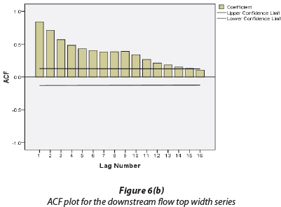
The ACF plots show that Lag 1 ACF for the series is close to 1 and the ACF has a linearly decreasing trend. Thus, to develop ARIMA models for discharge and top width series only first-order differencing is considered. Models with different numbers of autoregressive terms and moving average terms are fitted to the data series by applying SPSS package. BIC and R2 value for different models are compared and the model with the lowest value for BIC is selected. The ARIMA model with parameters (2,1,2) was found to be the best performing model for forecasting downstream discharge, and ARIMA (1,1,1) was found to be the best model for forecasting flow top width at the downstream river section. The discharge and top width forecasting models are obtained as:
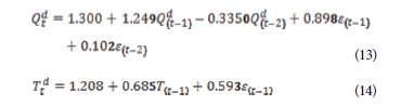
BIC and R2 value for the best discharge and top width forecasting models were found to be 10.354, 0.93 and 10.11, 0.91, respectively. ANFIS and ARIMA model performances were also evaluated using the same statistical criteria described earlier.
Results for the ANFIS and ARIMA models in forecasting downstream discharge and flow top widths are given in Table 3 and Figs 7 and 8.
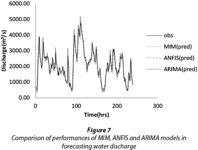
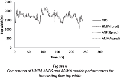
Performance parameters for the hybrid Muskingum model are given in Table 2. Discharge and/or top width data statistics for the gauging stations are given in Table 1. Comparing the results obtained in forecasting downstream values by using the models, it can be seen that the ANFIS model performance in terms of 'RMSE' is the best when downstream discharges are forecast, while the ARIMA model gives the best performances when downstream top widths are forecast. Performance of the hybrid Muskingum model closely follows performances of the ANFIS and ARIMA models. Considering average value of the observed flow and flow top width series for the downstream station, RMSE for forecasting downstream discharges in terms of percentage of the average downstream observed discharge value is 6.6%, 5.75% and 6.15% for HMIM, ANFIS and ARIMA models, respectively, and 5.53%, 5.39% and 5.30% when the downstream flow top widths are forecast. The results obtained show that the RMSE, representing an average prediction error, is less than 7% of the corresponding average observed value and indicates satisfactory performances by the HMIM, ANFIS and ARIMA models. Comparing the results given in Table 3 and Figs 7 and 8, it is seen that performance of the hybrid multiple inflow model is similar to that of the ANFIS and ARIMA models, in almost all counts considered in the study. The results obtained in the present study demonstrate the efficiency of the models in simulating and forecasting downstream flow top width in a river system.
DISCUSSION AND CONCLUSIONS
The present study indicates that for a river section, depending on the shape characteristics, there exists a relationship between depth of flow and flow top width at a section. Such relationship, when used in conjunction with the depth-discharge relationship, eventually results in a functional relationship/model involving top width and discharge variables for a section. The power law based top width-discharge model is in full agreement with the established depth-discharge model for sections with flow depth-top width relationships satisfying a power-law or linear relationship. A single power-law based rating curve may be adequate to describe top width versus discharge relationships when the flow depth is less than the bank-full depth; however, when the flow depth exceeds the bank-full depth a single rating curve may not give good results as the roughness and other flow conditions would vary widely. In that case, compound rating curves (Jain, 2008) having different segments in the curve described by different power law/other equations may be adopted to improve the model performances.
In the present study it is assumed that the top width-discharge relationship as given in Eq.(3) is single valued and provides a unique estimated value for the discharge corresponding to a given value of top-width at the section. Such estimates refer to the values of a discharge variable and, if used in a flow model, preserve model characteristics without violating any underlying principle. The hybrid multiple inflows Muskingum model obtained by using downstream flow top width variables represents a form of the multiple inflows Muskingum model, and describes flood wave movement in a river system as given by the Muskingum principle. The hybrid model formulations, ANFIS and ARIMA, have the advantage that they can provide downstream flow top width values estimated/forecast on the basis of upstream flow rates. The models are equipped with forecasting capabilities, can provide an estimate for downstream flow top width values in advance and are useful for real-time applications.
Results obtained in the study show that performances of the hybrid Muskingum model, ANFIS and ARIMA models were satisfactory, having errors of less than 7% of the average value of the observed series. The study also shows that power-law relationship involving section characteristics can describe the top width versus discharge relationship for a river section. Model application to the studied river system demonstrated the suitability of the ANFIS, ARIMA and hybrid Muskingum models in predicting downstream flow top width on the basis of several upstream flow/flow depth values in a river system.
ACKNOWLEDGMENTS
The authors would like to thank the Central Water Commission (CWC), Shillong for supplying the data. We are also highly thankful to DST (SERC) and the Indian Statistical Institute, Kolkata, for giving full assistance in carrying out the study.
REFERENCES
ANDERSON MG and BATES PD (2000) Evaluating 1D and 2D dimensional models for floodplain inundation mapping. Interim Report 007, United States Army. European Research Office of the US Army, London, England. [ Links ]
BALAZ M, DANACOVA M and SZOLGAY J (2010) On the use of the Muskingum method for the simulation of flood wave movements. Slovak J. Civ. Eng. 18 (3) 14-20. [ Links ]
BAZARTSEREN B, HILDEBRANDT G and HOLZ KP (2003) Short-term water level prediction using neural network and neuro-fuzzy approach. Neurocomputing55 (3-4) 439-450. [ Links ]
BISHT DCS and JANGID A (2011) Discharge modeling using adaptive neuro-fuzzy inference system. Int. J. Adv. Sci. Technol. 31 99-114. [ Links ]
BJERKLIE DM, MOLLER D, SMITH LC and DINGMAN SL (2005) Estimating discharge in rivers using remotely sensed hydraulic information. J. Hydrol. 309 191-209. [ Links ]
BOX GEP and JENKINS GM (1976) Time-series analysis: Forecasting and control. Holden Day Inc., San Francisco. [ Links ]
CHEN SH, LIN YH, CHANG LC and CHANG FJ (2006) The strategy of building a flood forecast model by Neuro-fuzzy network. Hydrol. Proc. 20 1525-1540. [ Links ]
CHOUDHURY P, SHRIVASTAVA RK and NARULKAR SM (2002) Flood routing in river networks using equivalent Muskingum inflow. J. Hydrol. Eng. 7 (6) 413-419. [ Links ]
CHOUDHURY P (2007) Multiple inflows Muskingum routing model. J. Hydrol. Eng. 12 473-481. [ Links ]
DASTORANI MT, MOGHADAMNIA A, PIRI J and RICO-RAMIREZ M (2009) Application of ANN and ANFIS models for reconstructing missing flow data. Environ. Monit. Assess. DOI: 10.1007/ s10661-009-1012-8. [ Links ]
FERNANDEZ N, JAIMES W and ALTAMIRANDA E (2010) Neuro-Fuzzy modeling for level prediction for the navigation sector on the Magdalena River (Colombia). J. Hydroinformatics 12 (1) DOI:10.2166/hydro.2010.059. [ Links ]
GASIOROWSKI D (2009) Flood routing by the non-linear Muskingum model. Arch. Hydro-Eng. Environ. Mech. 56 (3-4) 121-137. [ Links ]
GILLES DW (2010) Application of numerical models for improvement of flood preparedness. Master's thesis, University of Iowa. [ Links ]
HASHMI HN, SIDDIQUI QTM, KAMAL MA, MUGHAL HR and GHUMMAN AR (2012) Assessment of inundation extent for flash flood management. Afr. J. Agric. Res. 7 (8) 1346-1357. [ Links ]
ILABOYA IR, ATIKPO E, ONAIWU DO, UMUKORO L and ZUGWU MO (2011) Application of flood flow routing as a predictive model for flood management and control. J. Appl. Technol. Environ. Sanit. 207-220 pp. [ Links ]
JACQUIN AP and SHAMSELDIN AY (2006) Development of rainfall-runoff models using Takagi-Sugeno fuzzy inference systems. J. Hydrol. 329 154-173. [ Links ]
JAIN SK (2008) Development of integrated discharge and sediment rating relation using a compound neural network. J. Hydrol. Eng. 13 (3) 124-131. [ Links ]
JANG JSR (1993) ANFIS: Adaptive network-based fuzzy inference system. Trans. Syst., Man Cybernetics 23 665-685. [ Links ]
KHAN MH (1993) Muskingum flood routing model for multiple tributaries . Water Resour. Res. 29 1057-1062. [ Links ]
KHASHEI M and BIJARI M (2010) An artificial network (p,d,q) model for time-series forecasting. Expert Syst. Appl. 37 479-489. [ Links ]
KUMAR ND (2011) Extended Muskingum method for flood routing. J. Hydro-Environ. Res. 5 127-135. [ Links ]
LIONG SY, LIM WH and PAUDYAL G (2000) River stage forecasting in Bangladesh: Neural network approach. J. Comput. Civ. Eng. 14 (1) 1-8. [ Links ]
MARTINS OTACHE Y, SADEEQ MA and AHANEKU IE (2011) ARMA modeling of Benue River flow dynamics: Comparative study of PAR model. Open J. Mod. Hydrol. 1 1-9. [ Links ]
McCARTHY GT (1937) The unit hydrograph and flood routing. Conference of North Atlantic Division, US Army Corps of Engineers, New London, CT. US Engineering. [ Links ]
O'DONNELL T (1985) A direct three-parameter Muskingum procedure incorporating lateral inflow. J. Hydraul. Eng. 30 479-496. [ Links ]
PAPPENBERGER F, MATGEN P, BEVEN KJ, HENRY JB and PFISHER L, DE FRAIOPONT P (2006) Influence of uncertain boundary conditions and model structure on flood inundation predictions. Adv. Water Resour. 29 (10) 1430-1449. [ Links ]
SRINIVAS N and DEB K (1994) Multiple objective optimizations using non-dominated sorting in genetic algorithms. Evol. Comput. 2 (3) 221-248. [ Links ]
VALIPOUR M, BANIHABIB ME and BEHABAHANI SR (2012) Parameters estimate of autoregressive moving average and auto-regressive integrated moving average models and compare their ability for inflow forecasting. J. Math. Stat. 8 (3) 330-338. [ Links ]
WANG Y, HAIDEN T and KANN A (2006) The operational limited area modeling system at
ZAMG: Aladin-Austria. Osterr. Beitrage Meteorol. Geophy. 37 33.
YANG K, LIU X, CAO S and HUANG ER (2013) Stage-discharge prediction in compound channels. J. Hydraul. Eng. DOI:10.1061/ (ASCE)HY.1943-7900.0000834. [ Links ]
YU D and LANE SN (2006) Urban fluvial flood modeling using a two-dimensional diffusion wave treatment, part 1: mesh resolution effects. Hydrol. Proc. 20 (7) 1541-1565. [ Links ]
ZHENG N, TACHIKAWA Y and TAKARA K (2008) A distributed flood inundation model integrating with rainfall-runoff processes using GIS and remote sensing data. Int. Arch. Photogram. Remote Sens. Spatial Inf. Sci. XXXVII (B4) 1513-1518. [ Links ]
NOTATIONS
The following symbols are used in this technical note:
c1, c2, c3 = Muskingum routing coefficients Δt = time-period
k = coefficient of storage having dimension of time and is approximately equal to flood wave travel time from the upstream point to the downstream point in the reach
x = relative importance of equivalent single inflow as compared with the outflow in making storage in the routing reach
 = Model generated outflow at time t + Δt
αp, βp = upstream section properties
α p,βd = downstream section properties
σp,r = shift factor associated for transfer of upstream flow from p to r or it represents the relative position of the pth gauging site with respect to the point of application of the single equivalent inflow, r
Qte,u,r = equivalent flow at a point r in the basin for n upstream flows at time t Qtu,p = flow at an upstream point p at time t
Qtd = outflow at the common downstream station of the river system at time t
Q(*) = instantaneous water discharge at a section (*) at time t
Tt(*) = instantaneous flow top width at a section at time t (*) = a section
n = number of variables
c = number of categories per variable
a , b = inputs for ANFIS model
z = output for ANFIS model
pi, qi, ri = linear parameters in Sugeno-fuzzy model
l, d, q = parameters in the ARIMA model
Received 29 January 2013
Accepted in revised form 10 June 2014.
* To whom all correspondence should be addressed.+9085228262; e-mail: nazrinullah@gmail.com

