


Serviços Personalizados
Artigo
 Inglês (pdf)
 Artigo em XML
 Referências do artigo
Indicadores

Links relacionados
-
 Citado por Google
 -
 Similares em Google
Compartilhar

 Permalink
Water SA
versão On-line ISSN 1816-7950
versão impressa ISSN 0378-4738
Water SA vol.39 no.3 Pretoria 2013
TECHNICAL NOTE
A model to assess water tariffs as part of water demand management
JJ Hoffman*; JA du Plessis
Stellenbosch University, Department of Civil Engineering, P/Bag X1, MATIELAND, 7602, South Africa
ABSTRACT
Water Conservation and Water Demand Management (WC/WDM) forms part of integrated water resource management and can be used as an economically viable alternative to the upgrade of infrastructure to balance supply and demand. In order to enable effective decision-making, a model was developed in this study to estimate expected water savings and the financial impact of a change in water tariff as a WC/WDM measure. This paper describes a model that was developed for municipalities to calculate the predicted change in water use and the associated income. The model takes into account variation in price elasticity per tariff block. The effectiveness of the model as a planning tool is illustrated through an appropriate example.
Keywords: water demand management, price elasticity, change in water tariff, block tariff, WC/WDM model
INTRODUCTION
Limited water supplies and increasing water demands mean that the effective management of water resources has become much more important now than in the past. The implementation of WC/WDM projects is usually used as a crisis management tool to reduce immediate water shortage and to allow time for the planning and construction of infrastructure to increase water supply. In the current economic climate, it is however important to incorporate WC/WDM into integrated water resource management and to evaluate WC/WDM as an economically viable option.
Different models (e.g. as presented by Hoffman, 2011) are available to evaluate WC/WDM options. Some of these models focus on the economic evaluation of WC/WDM options while others estimate the impact that the implementation of different WC/WDM options have had or will have on water consumption. Economic evaluation models include aspects such as the deferral of capital, economic sustainability and calculation of unit reference values (URV), while the implementation models have focused on the impact WC/WDM projects such as meter replacement (Noss et al., 1987), pressure management and leak detection have had or will have on water consumption and income.
Jansen and Schulz (2006) focused on the evaluation of the factors influencing WC/WDM, i.e., climate, revenue and pricing. Regression analysis was done on the impacts thereof and price elasticity was calculated based on these values. No attempt was however made to quantify the economic impact a change in a block water tariff has on price elasticity. Nataraj and Hanemann (2011) analysed the impact of the introduction of a third price block on residential water consumption in Santa Cruz, and concluded that consumers who expected to face the higher marginal price in the 3rd block would reduce their consumption.
This paper presents a novel, robust WC/WDM model that was developed to estimate the change in consumption as well as the expected revenue due to a change in water tariff. The model takes into account a block tariff structure and incorporates the possibility that consumers will react differently to tariff increases depending on their current consumption patterns. In their study, Klaiber et al. (2013) presented a similar estimation of water consumption with a 2-block pricing structure incorporating monthly and seasonal variations. Data related to all of the variations in their model are not necessarily available from relatively small South African municipalities. The model presented in this paper was however developed for a 6-block pricing structure and allows for limited available input data from municipalities. An example was used to illustrate the impact of a change of water tariff on consumption as well as the associated revenue for municipalities.
Changing the water tariff
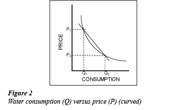
The relationship between the cost of water and consumption is described as price elasticity. Price elasticity can be illustrated with the use of a combination of different graphs, presented in Figs. 1 to 3. The relationship in its simplest form can be presented as a linear relationship - consumption (Q) linearly decreases as the price of water (P) increases. The relationship may also be represented by an arc illustrated in Fig. 2 (Veck and Bill, 2000). In this representation, the consumption gradually decreases as the price increases.

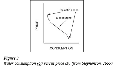
Stephenson (1999) suggested that the best way to represent the relationship is by 3 well-defined regions, presented in Fig. 3. This graph consists of an elastic zone and 2 inelastic zones. In the elastic zone, it is very easy for the consumer to adjust their consumption. As the cost decreases, the consumption increases. Subsequently, as the cost increases, it becomes harder to reduce consumption at the same rate as before and, thus, the inelastic zone results. There is however a minimum required consumption for each consumer. The relationship thus becomes inelastic at a specific point and a price increase has no further impact on the consumption above this level. On the other side of the spectrum, a reduction in the price causes an increase in water consumption. Again it reaches a point where the consumer can only consume a specific maximum amount of water and a further reduction of the cost will not result in an increase in consumption. This forms the second inelastic zone.
Price elasticity can be calculated as follow (Van Vuuren et al, 2004):

where:
e = Price elasticity
P = Price of water (R/kℓ, with R expressed in ZAR)
Q = Water consumption (kℓ) dP = Change in consumption dQ = Change in price
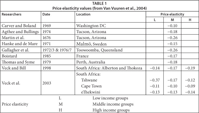
Several research studies have been conducted on price elasticity. Table 1 (Van Vuuren et al., 2004) shows a summary of some of these studies. From Table 1, the average price elasticity values range between -0.1 and -0.2. This means that if the price of water increases by 20%, and a value of -0.15 for price elasticity is adopted, then a reduction of 3% in water consumption can be expected (applying Eq. (1)).
Modelling the expected consumption due to a change in tariff
The impact of a water tariff change, along with the change in the expected revenue from water sales, form the key components of the model developed herein. According to Eq. (1), this calculation should be simple as long as the rate of change of the water consumption (P) remains constant. This is however not the case where municipalities make use of a block tariff system. A good block tariff structure means that the tariff for basic water is lower than the subsequent tariff blocks corresponding to higher consumption. The principle is that a consumer will pay more per kilolitre if more water is used than what is required for basic use. It is therefore essential that any model that is used to predict the impact of a change in water tariff must take into account these variations in the tariff blocks as well as the monthly variation in the consumption by different water users. These data are not always available and the distribution of different user groups frequently needs to be estimated.
The model presented in this study was set up in a Microsoft Excel spreadsheet and allows for different elasticity values for each tariff block. In the model, water users are categorised according to the maximum tariff block in which their average water consumption falls. The volume of water used is then calculated for each block. In the model, the price elasticity value for each tariff block is then applied to calculate the estimated change in usage. Such a variation in elasticity values for each tariff block is necessitated due to the fact that a consumer's willingness to reduce their consumption can differ between consumers in the 0 kℓ - 6 kℓ block and those in the higher blocks. A consumer who uses 100 kℓ per month (which falls in a higher tariff block) will be able to save more than a consumer who only uses the basic consumption (0 kℓ - 6 kℓ) in the lowest block. Equation (1) is used to calculate the water savings of each block. Due to these savings, some consumers will now fall within a lower block. This is taken into account before the expected revenue is calculated. The revenue from the new (reduced) water consumption is calculated and compared with the water saving.
The following input parameters are required for the model:
- The total number of consumers
- Allocation of water users per block
- Annual water consumption of each user
- Annual revenue from water sales before tariff change
- Block tariff structure
- Price of water for each of these blocks before tariff change
- Proposed price adjustment
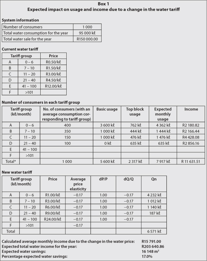
The following example will serve to illustrate the working of the model: A municipality provides water to 1 000 customers. The total annual consumption is 95 000 kℓ with a total annual revenue from water sales of R150 000. The municipality uses a block tariff structure with 5 blocks. The average monthly water consumption of the maximum water consumption falls consumers is distributed as follows: 400 consumers' in Block A (lowest tariff), 350 consumers in Block B, 150 consumers in Block C, 100 consumers in Block D and no consumers in Block E (highest tariff). The municipality is planning on doubling the tariffs of each block and needs to make an estimate on the expected drop in consumption and impact on revenue due to these changes. The model is used to assess the impact of the doubling of the tariffs and the results are presented in Box 1. The calculation procedures used in the model are illustrated through a step-by-step discussion of the example.
The 'System information' and 'Current water tariff' contains the user-defined input for the specific case study. The model allows for a maximum of 6 levels in the block tariff structure. In the case of the example, only 5 levels are used. For this example, the block tariff categories (0-6, 7-10, 11-20, 21-40, 41-100) are used along with the associated tariff structures (R0.50, R1.50, R3.00, R4.50, and R12.00) in R/kℓ.
The 'Number in each tariff group' section within Box 1 illustrates how the model calculates usage and revenue in each block. The 'N consumers' represent the average monthly number of consumers that use a maximum volume of water within each block.
The 'Basic usage' represents the total volume of water used by consumers who exceed the maximum limit in the respective blocks. For example, in Block B there are 350 consumers, 150 in Block C and 100 in Block D. To calculate the basic usage for each block, the consumers in all the blocks below the block under consideration need to be added together and multiplied by the consumption per block (For Block C, the consumption amounts to 20-10 = 10 kℓ). This reflects the situation where it is known that if a consumer falls within Block C, the model uses 6 kℓ falling in block A and 4 kℓ in Block B. Therefore the basic usage for Block C (1 000 kℓ) in the example represents the sum of the 100 consumers using water falling in Block D * 10 kℓ; the basic usage in Block B (1 000 kℓ) amounts to 250 (100 consumers in Block D + 150 consumers in Block C) * 4 and 600 (100 + 150 + 350) * 6 for Block A (3 600 kℓ). The basic usage for higher block users is known from the above, but not the average usage of the consumers that fall in a specific tariff block. For example, the consumers in Block B use at least 6 kℓ each (which is the consumption in the lower Block A), but it is still unknown how much water they use in Block B. It is somewhere between 6 and 10 kℓ per month. This is defined as the 'Top block usage' as illustrated in 'Number in each tariff group' section within Box 1.
To estimate the 'Top block usage' in the model, the following steps can be employed. Since the 'Total water consumption for the year' (95 000 kℓ) is known, and the total of the 'Basic usage' can easily be calculated (5 600 kℓ), it is possible to calculate the total 'Top block usage'. The average monthly consumption is 7 917 (i.e. 95 000 kℓ /12 months). Therefore the 'Top block usage' amounts to 2 317 k£ (7 917 kℓ - 5 600 kℓ).
An assumption is made that the 'Top block usage' is proportionally redistributed to the different blocks according to the available consumption per block. For example Block B's maximum consumption is 350 x 4 = 1 400 kℓ. Similarly the maximum consumption in Block A is 2 400 kℓ, Block C is 1 500 kℓ and Block D is 2 000 kℓ with a total of 7 300 k (2 400 kℓ + 1 400 kℓ + 1 500 kℓ + 2 000 kℓ) for this example.
The 'Top block usage' in Block B can be calculated to be equal to 444 kℓ (1 400/7 300 x 2316).
The 'Expected monthly usage' in Box 1 represents the total of the 'Basic usage' and 'Top block usage', while the 'Expected monthly income' represents the monthly revenue calculated using the sale of the 'Expected monthly usage' per block multiplied by the applicable block tariff.
The 'Total *' value in Box 1 represents the total of each column. The 'consumer' and the total sum of the 'Expected monthly usage' must match the values in the 'System Information'. The total of 'Expected monthly income' and the information in 'System Information' do not necessarily match, due to the possible error distributions of 'consumer' and 'Add usage'. These differences will be dealt with separately in the model.
The 'New water tariff' section within Box 1 illustrates how the change in consumption is calculated in the model using the new tariff for each block and applying the average price elasticity for each block. In the example, the tariff for each block is doubled and the same average price elasticity for all the blocks is used. The other variables are calculated as follows:
- dP/P
This represents the change in price as a proportion to the original price. Block A is therefore 1 [(R1.00 - R0.50) / (R0.50)].
- dQ/Q
This represents the change in consumption as a proportion to the original consumption calculated according to the price elasticity equation (Eq. (1)), as discussed. For Block A it amounts to -0.17 (-0.17 x 1).
- Qn
This represents the new 'Expected monthly consumption' due to the impact of the tariff adjustments. Qn for each block is calculated as follows:
- The average water consumption of each of the 'consumer' in the tariff block is calculated.
- The price elasticity of each block is applied to the average consumption of the consumers in the applicable block and a new consumption is calculated.
- The 'Expected monthly consumption' (Qn) for each block is calculated.
The model then calculates the expected average monthly water use and expected annual revenue after the implementation of the changes in the tariffs. In the example the expected monthly revenue amounts to R15 791.00 as illustrated in Box 1, with the expected annual revenue R203 640.86. In calculating the annual revenue an adjustment is made to take into account the differences between the calculated monthly water sales and actual sales. The 'Expected total water revenue for the year' (R203 640.86) is calculated by increasing the current water sale (R150 000.00) with the ratio of 'Calculated average monthly revenue due to the change in the water price' over 'Total expected monthly income' (R16 791.00/R12416.67).
Finally, the model calculates the total savings, as a percentage, due to the change in water tariff. In the example presented the saving is 17%, which is the same as the elasticity value (e = -0.17), assumed to be constant for all the blocks.
APPLYING THE MODEL TO A HYPOTHETICAL CASE STUDY
The City of Cape Town proposed a 9% water tariff increase for each tariff block for the 2010/11 financial year (City of Cape Town, 2010). A hypothetical case, based on a similar increase, is presented below. The model was applied to estimate alternative residential tariff increases and to investigate the effect it could have on water savings and revenue.
The following assumptions were made in the model.
- For the purpose of this example an increase of 10% was assumed and further increases in steps of 5% were investigated.
- Domestic consumers with a block tariff of 6 levels or less were used in the analysis.
- The analysis was done for 1 000 representative consumer units with an average monthly consumption of 25.4 kℓ/ month.
- The distribution of consumers and block tariffs presented in Table 2 were used.
- The water tariffs for the City of Cape Town's financial year 2009/10 (City of Cape Town, 2010) were used and the water tariff was then increased with 5%, 10%, 20%, etc.
- The average price elasticity values for low-, medium- and high-revenue groups, presented in Box 1, were used for different tariff blocks as follows: low revenue elasticity values were used in tariff blocks A and B; middle-income elasticity values for tariff blocks C and D; tariff block E represented the high-income elasticity values.
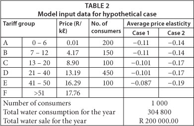
Two possible scenarios were analysed for the case study. In the first scenario, the price elasticity values from Table 1 (Van Vuuren et al., 2004) for Cape Town (-0.11, -0.10, -0.09) were used. In the second scenario, values from Table 1 (Van Vuuren et al., 2004) for South Africa (-0.14, -0.17, -0.19) were used.
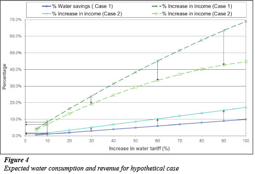
The estimated percentage water savings as well as the percentage increase in revenue were calculated by the model for every set of alternative new tariffs. The impact of these new tariffs for the two different elasticity values is illustrated in Fig. 4.
CONCLUSIONS
The model presented in this paper took into account variation in price elasticity per tariff block. The effectiveness of the model as a planning tool is illustrated through an appropriate example. A number of different conclusions can be made:
- An increase in water tariffs causes an increase in the expected water savings and therefore causes a reduction in water consumption. The price elasticity values selected determines the slope of the decrease in water consumption, as could be expected.
- The percentage of water savings and revenue increases with an increase in the absolute elasticity values for a specific increase in water tariffs. The percentage increase in revenue from water sales is typically higher than the actual percentage in water savings. Using the correct price elasticity values is essential to determine the correct expected impacts of price increases.
The proposed model is able to analyse the possible impact of an increase in water tariffs on the water consumption and associated income. It can be concluded that the savings gained from water tariff increase may not be significant unless notable price elasticity values apply in the area. Water saving is typically lower than the increase in revenue induced by the increased cost and therefore the water saving could be regarded as a secondary benefit.
This paper was originally presented at the 2012 Water Institute of Southern Africa (WISA) Biennial Conference, Cape Town, 6-10 May 2012.
REFERENCES [ Links ]
HOFFMAN JJ (2011), Ekonomiese Besluitnemingskriteria vir Water-aanvraagbestuur & Waterbesparing. MSc thesis, University of Stellenbosch. [ Links ]
JANSEN A and SCHULZ C (2006) Water demand and the urban poor: A study of the factors influencing water consumption among households in Cape Town, South Africa. S. Afr. J. Econ. 74 (3) 11-14. [ Links ]
KLAIBER HA, SMITH VK, KAMINSKY M and STRONG A (2012) Measuring Price Elasticities for Residential Water Demand with Limited Information. NBER Working Paper No. 18293, August 2012. National Bureau of Economic Research, Cambridge. [ Links ]
NATARAJ S and HANEMANN WM (2011) Does marginal price matter? A regression discontinuity approach to estimating water demand. J. Environ. Econ. Manage. 61(2) 198-212. [ Links ]
NOSS RR, NEWMAN GF and MALE JW (1987) Optimal Testing Frequency for Domestic Water meters. J. Water Resour. Plann. Manage. 113 (1) 1-14. [ Links ]
STEPHENSON D (1999) Demand management theory. Water SA 25 (2) 115-121. [ Links ]
VAN VUUREN DS, VAN ZYL HJD, VECK GA and BILL MR (2004) Payment Strategies and Price Elasticity of Demand for Water for Different revenue Groups in Three Selected Urban Areas. WRC Report No. 1296/1/04. Water Research Commission, Pretoria. [ Links ]
VECK GA and BILL MR (2000) Estimation of the Residential Price Elasticity of Demand for Water by Means of the Contingent Valuation Approach. WRC Report No. 790/1/00. Water Research Commission, Pretoria. [ Links ]
* To whom all correspondence should be addressed. +27 21 808-4358; e-mail: hoffmann@sun.ac.za

