Development of a customised design flood estimation tool to estimate floods in gauged and ungauged catchments

 

 

OJ Gericke^{I, II, *}; JA du Plessis^II

^IFaculty of Engineering and Information Technology, Department of Civil Engineering, Central University of Technology, Free State, South Africa
^IIDepartment of Civil Engineering, University of Stellenbosch, P/Bag X1, Matieland 7602, South Africa

 

 

---

ABSTRACT

The estimation of design flood events, i.e., floods characterised by a specific magnitude-frequency relationship, at a particular site in a specific region is necessary for the planning, design and operation of hydraulic structures. Both the occurrence and frequency of flood events, along with the uncertainty involved in the estimation thereof, contribute to the practising engineers' dilemma to make a single, justifiable decision based on the results obtained from the plethora of 'outdated' design flood estimation methods available in South Africa. The objectives of this study were: (i) to review the methods currently used for design flood estimation in South Africa for single-site analysis, (ii) to develop a customised, user-friendly Design Flood Estimation Tool (DFET) containing the latest design rainfall information and recognised estimation methods used in South African flood hydrology, and (iii) to demonstrate the use and functionality of the developed DFET by comparing and assessing the performance of the various design flood estimation methods in gauged catchments with areas ranging from 100 km² to 10 000 km² in the C5 secondary drainage region, South Africa. The results showed that the developed DFET will provide designers with an easy-to-use software tool for the rapid estimation and evaluation of alternative design flood estimation methods currently available in South Africa for applications at a site-specific scale in both gauged/ungauged and small/large catchments. In applying the developed DFET to gauged catchments, the simplified 'small catchment' (A < 15 km2) deterministic flood estimation methods provided acceptable results when compared to the probabilistic analyses applicable to all of the catchment sizes and return periods, except for the 2-year return period. Less acceptable results were demonstrated by the 'medium catchment' (15 kirf < A < 5 000 kirf) deterministic and 'large catchment' (> 5 000 km2) empirical flood estimation methods. It can be concluded that there is no single design flood estimation method that is superior to all other methods used to address the wide variety of flood magnitude-frequency problems that are encountered in practice. Practising engineers' still have to apply their own experience and knowledge to these particular problems until the gap between flood research and practice in South Africa is narrowed by improving existing (outdated) design flood estimation methods and/or evaluating methods used internationally and developing new methods for application in South Africa.

Keywords: Design flood, design rainfall, estimation, ungauged catchments, flood magnitude-frequency

---

 

 

Introduction

The estimation of design flood events, i.e., floods characterised by a specific magnitude-frequency relationship, at a particular site in a specific region is necessary for the planning, design and operation of hydraulic structures (Pegram and Parak, 2004). In essence, the failures of these structures caused by floods are largely due to the immense variability in the flood response of catchments to rainfall, which is innately variable in its own right (Alexander, 2001). Consequently, design flood estimations are likely to display relatively wide magnitude-frequency bands of uncertainty (Alexander, 2002). Thus, both the occurrence and the frequency of flood events, along with the uncertainty involved in the estimation thereof, contribute to the practising engineers' dilemma to make a single, justifiable decision based on the results obtained from the plethora of 'outdated' design flood estimation methods available in South Africa.

Most of these 'outdated' design flood estimation methods were developed in the 1970s, with some still reliant on graphical procedures. The recent (2006) compilation of the South African National Roads Agency Limited (SANRAL) Drainage Manual, which is regarded by many practising engineers' as an authoritative reference document, also proposes the use of a suite of design flood estimation methods with associated graphical procedures. However, there is no guarantee that these time-consuming methods using graphical input would result in more acceptable flood magnitude-frequency relationship results compared to the results obtained with more simplified methods, e.g., the Rational method (RM). In addition, the degree of uncertainty in terms of these methods' relative applicability, based on their basic assumptions, has not been evaluated.

In order to overcome some of the inherent limitations of the currently-used methods in terms of their user-friendliness, and to enhance the practicing engineers' decision-making process, the Utility Programs for Drainage (UPD) software (Van Dijk, 2005) was developed to complement the Drainage Manual. The UPD software consists of a number of easy to use, state-of-the-art, user-friendly programs for the hydraulic design and analysis of drainage structures. In terms of flood hydrology, it is limited to flood estimations based on deterministic, empirical and probabilistic methods. However, the estimation of catchment parameters (e.g. average catchment and main watercourse slopes, slope frequency distribution classes and main watercourse longitudinal profiles) is not possible in UPD, while the design rainfall information is limited to Adamson's (1981) TR102 daily design rainfall database used in conjunction with the modified Hershfield equation (Alexander, 2001).

This paper attempts to provide preliminary insight into the current suitability of the various methods used in South Africa to estimate the design flood, by using an integrated Design Flood Estimation Tool (DFET) developed by Gericke (2010), which revolves around the basic acceptance that there is no single design flood estimation method that is superior to all other methods under the wide variety of flood magnitude-frequency problems that will be encountered in practice. Apart from the inclusion of recognised design flood estimation procedures, the DFET also provides a powerful data management framework with a consistent, intuitive platform for organising and analysing both catchment parameters and design rainfall information. To date, the latter functionalities (catchment parameter and design rainfall estimation using the latest methodologies) are not available in any of the software used to estimate design floods in South Africa.

The objectives of the study reported in this paper are discussed and explained in the next section, followed by an overview of the study area's spatial distribution and characteristics. Thereafter, the methods used in South Africa to estimate the design flood are reviewed in detail. The methodologies involved in assessing the objectives are then expanded on in detail, followed by the results, discussion and conclusions.

 

Objectives of study

The objectives of this study were: (i) to review the methods currently used for design flood estimation in South Africa for single-site analysis, (ii) to develop a customised, user-friendly DFET containing the latest design rainfall information and recognised estimation methods used in South African flood hydrology, while taking cognisance of the practising engineer's dilemma to make a single, justifiable decision using the plethora of 'outdated' design flood estimation methods locally available, and (iii) to demonstrate the use and functionality of the developed DFET, by comparing and assessing the performance of the various design flood estimation methods in gauged catchments with areas ranging from 100 km² to 10 000 km2 in the C5 secondary drainage region, South Africa.

A number of assumptions in recognition of the current status quo of South African flood hydrology were made in this study. Firstly, it was assumed that a large percentage of civil engineers tend to use only well-known and simplified 'small catchment' design flood estimation methods (e.g. the 157-year old RM) beyond their recommended areal limitations. In other words, not all engineers involved in design flood estimation in South Africa can be regarded as 'leading consulting engineering hydrologists', irrespective of their applied contributions in the field of flood hydrology, stormwater management and road drainage in both small and large catchments. Secondly, it was accepted that the use of more complex design flood estimation methods, e.g., the Synthetic Unit Hydrograph (SUH), with associated time-consuming graphical estimation procedures in larger catchment areas, does not necessarily result in a satisfactory estimation of flood magnitude-frequency relationships. Lastly, the reality that practising engineers do not always have the opportunity to compare probabilistic flood estimation results in a gauged catchment with that of rainfall-based methods in ungauged, small catchments, in order to justify their results, was recognised. It is envisaged that the developed DFET will enable the rapid estimation and evaluation of alternative design flood estimation methods at a site-specific scale in both gauged/ungauged and small/large catchments. However, the DFET's data management framework is such that practitioners will still have to apply their own experience and knowledge to a particular flood magnitude-frequency problem.

 

Study area

South Africa is demarcated into 22 primary drainage regions, which are further delineated into 148 secondary drainage regions. The study area is situated in primary drainage region C and comprises of the C5 secondary drainage region (Midgley et al., 1994). As shown in Fig. 1, the study area covers 34 795 km² between 28°25' and 30°17' S and 23°49' and 27°00' E, and is comprised of 99.1% rural areas, 0.7% urbanisation and 0.2% water bodies (DWAF, 1995). The natural vegetation is dominated by Grassland of the Interior Plateau, False Karoo and Karoo. Cultivated land is the largest human-induced vegetation alteration in the rural areas, while residential and suburban areas dominate the urban areas (CSIR, 2001). The topography is gentle with slopes between 2.4% and 5.5% (USGS, 2002), while water tends to pond easily, thus influencing the attenuation and translation of floods. The mean annual precipitation (MAP) is 424 mm, ranging from 275 mm in the west to 685 mm in the east (Lynch, 2004), and rainfall is characterised as highly variable and unpredictable. The rainy season starts in early September and ends mid-April, with a dry winter. The Modder and Riet Rivers are the main river reaches and discharge into the Orange-Vaal River drainage system (Midgley et al., 1994).

Review of design flood estimation methods

Universally, 3 basic approaches to design flood estimation are available in South Africa, namely the probabilistic, deterministic and empirical methods (Alexander, 1990; 2001; Parak and Pegram, 2006; Van der Spuy and Rademeyer, 2010). In order to assess the uncertainty in flood estimation methods, all three approaches should, where possible and appropriate, be included in any specific design situation. The following sub-sections provide a review of the design flood estimation methods currently used in South Africa for single-site analyses.

Probabilistic methods

Design flood estimations using probabilistic methods entail the frequency analysis of observed flood peak data, from a flow-gauging site, that are adequate in both length and quality of data. The use of observed data in flood frequency analysis assumes that the data are stationary; however, frequently this is not the case, due to, inter alia, land cover and land-use changes within a particular catchment or region. Probabilistic methods may be used at a single site, or, preferably, a regional approach should be adopted (Smithers, 2012).

The objectives of probabilistic analysis are to (Alexander, 2001):

• Summarise the observed flood peak data;
• Estimate certain parameters; and
• Select and fit an appropriate theoretical probability distribution to the observed flood peaks with which exceedance probabilities can be estimated.

These listed objectives are subsequently discussed.

The summarisation of observed flood peak data includes the ranking of either the annual maximum series (AMS) or the partial duration series (PDS) in a descending order of magnitude, after which an exceedance probability is assigned to the plotted values. The AMS can be defined as the highest instantaneous peak streamflow value in each hydrological year for the period of record (Schulze, 1995; Chadwick and Morfett, 2004). In the PDS, the selection procedure entails that some of the monthly/annual maximum peaks may be excluded in the series using a threshold exceedance value (Kite, 1988). In cases where the number of ranked peak events is equal to the number of data years, the PDS is referred to as an annual exceedance series (AES). Various opinions regarding the use of the AMS and PDS have been expressed in the literature. According to Adamson (1981), the AMS are preferred to the PDS based on the ease of use, rather than on the theoretical efficiency in characterising the extreme value time series. On the other hand, the PDS is recommended for short data records, since the AMS could result in a considerable loss of information for the estimation of flood exceedance probabilities (Madsen et al., 1997); however, Reich (1963) highlighted that the AMS and PDS tend to converge for return periods longer than 10 years. In addition, the use of the PDS overcomes the objection that significant events, which are not the largest event in a specific year, are excluded from the analysis. Therefore, if the arrival rate of events is large enough, the PDS design estimates could be more accurate than the AMS (Stedinger et al., 1993). Despite the advantages of the use of the PDS and apart from the research conducted by Gorgens (2007), the use of the PDS has made very little impact on South African flood hydrology practice.

Plotting position formulae (Eq. (1)) are commonly used in South Africa to assign an exceedance probability to flood peaks. It is based on the assumption that if (n) values are distributed uniformly between 0% and 100% probability, then there must be (n + 1) intervals, (n - 1) intervals between the data points and 2 intervals at the ends (Chow et al., 1988; SANRAL, 2006).

where:

T = return period (years)

a = constant (Table 1)

b = constant (Table 1)

m = number, in descending order, of the ranked events (peak flows)

n = number of observations/record length (years)

 

 

Cunnane (1978) investigated the various available plotting position methods using unbiasedness criteria and minimum variance criteria. An unbiased plotting method for equally-sized samples is defined as the average of the plotted points for each value of m falling on the theoretical distribution line. A minimum variance plotting method minimises the variance of the plotted points about the theoretical line. The findings of Cunnane (1978), based on the above criteria, indicate that different plotting position formulae (Table 1) are applicable to different theoretical probability distributions (Chow et al., 1988). However, the Cunnane formula is generally used in South Africa, and is also being recommended by the Department of Water Affairs (DWA) (Van der Spuy and Rademeyer, 2010).

Parameter estimation methods available for fitting theoretical probability distributions to observed flood peak values include the Linear Moments (LM), Maximum Likelihood (ML), Method of Moments (MM), Probable Weighted Moments (PWM) and Method of Least-Squares (MLS) (Yevjevich, 1982; Chow et al., 1988; Kite, 1988; Stedinger et al., 1993). All these methods will, within limits, estimate the parameters of a theoretical probability distribution from a particular data sample (Kite, 1988). LM estimators are used extensively internationally as a standard procedure for flood frequency analysis, screening for discordant data and testing clusters for homogeneity (Smithers and Schulze, 2000a). Some caution and criticism of the use of LM is also evident in the literature. Alexander (2001) cautions that LM are too robust against outliers and emphasised that both low and high outliers are important characteristics of the flood peak maxima. The suppression of the effect of outliers could result in unrealistic estimates of longer return period values. Therefore, further investigation of LM for possible general use in South Africa is necessary (Smithers, 2012). Alexander (1990, 2001) recommends either MM or PWM estimators for probability distribution fitting in South Africa, either at a single site or when a regional approach is adopted.

The fitting of an appropriate theoretical probability distribution to a data set provides a compact and smoothed representation of the frequency distribution revealed by the limited information available and enables the systematic extrapolation to frequencies beyond the data set range (Smithers and Schulze, 2000a). The question of selecting an appropriate distribution has received considerable attention in the literature, with diverging opinions expressed in the international literature (Smithers, 2012). Schulze (1989) highlighted that variations due to the season, storm type and duration and regional differences could impact on the selection of a single suitable probability distribution and questioned the accuracy thereof. Beven (2000) emphasised that different probability distributions may fit the observed values well, but are seldom comparable when extrapolated, while the use of relatively short records only represents a small sample of the possible floods at a particular flow-gauging site.

Van der Spuy and Rademeyer (2010) recommend the Log-Normal (LN), Log-Pearson Type 3 (LP3) and General Extreme Value (GEV) probability distributions for flood frequency analysis at a single site in South Africa; while Gorgens (2007) regarded both the LP3 and GEV probability distributions as the most appropriate to be used locally. Alexander (1990, 2001) limits his recommendation to the LP3 probability distribution for design flood estimation in South Africa. In the United States of America (USA) the LP3 probability distribution is accepted as being the most general and objective distribution (Stedinger et al., 1993), while the Institute of Hydrology (IH) (IH, 1999) recommends the use of the General Logistic (GLO) distribution based on LM estimators in the United Kingdom (UK).

Taking cognisance of the fact that frequently no or inadequate observed flood peak data might be available at a single site, the use of regional flood frequency analysis may be necessary. In essence, regional flood frequency analysis is based on the assumption that the standardised variate distributions of flood peak data are similar at every single site in a homogeneous region and that the data from various single sites, after appropriate site-specific scaling, can be combined to generate a single regional flood frequency curve representative of any site in that region (Smithers and Schulze, 2003). However, this paper's literature review focuses on the use of design flood estimation methods at a single site, with the anticipated focus user group for the developed DFET comprising of general civil engineering technicians, engineering technologists and engineers employed at consultancies, who are not necessarily specialists in the field of flood hydrology who would be more likely to follow a regional approach.

The following theoretical probability distributions fitted using MM parameter estimation procedures are included as options in the DFET:

• Normal
• LN
• LP3
• GEV distributions

The GLO distribution based on LM parameter estimators is also included in the DFET to propagate the potential use and further investigation thereof in South Africa, due to the wide application internationally. However, the aim should be to fit all theoretical distributions using the same parameter estimator. A detailed description (probability density function, assumptions and limitations) of these theoretical probability distributions is listed in Table A1 of Appendix A.

Deterministic methods

In the application of deterministic methods, all complex, heterogeneous catchment processes are lumped into a single process to enable the estimation of individual design flood events in a simple and robust manner (IH, 1999). The event-based approach of deterministic methods greatly simplifies the estimation of catchment conditions prior to the occurrence of a flood event, while endeavouring to estimate the expected result (runoff) from causative factors (rainfall), based on the assumption that the frequency of the estimated runoff and the input rainfall is equal, while being influenced by catchment representative inputs and model parameters (Smithers, 2012). In simplistic terms, the T-year recurrence interval rainfall will produce the T-year flood, if the catchment is at average condition. Thus, the task concerns transforming excess rainfall for the T-year design storm into T-year flood runoff. This assumption considers the probabilistic nature of rainfall, but the probabilistic behaviour of other inputs and parameters is ignored. Thus, by ignoring the direct implications of joint probability, deterministic methods generally assume that the catchment is in an 'average' state in order to generate the T-year flood from the T-year rainfall event (Pilgrim and Cordery, 1993; Alexander, 2001; Rahman et al., 2002).

Taking into consideration the vast complexity and spatial and temporal variability of catchment processes and their driving forces, as well as the probable significant bias introduced by ignoring the joint probability of rainfall and runoff, it is not surprisingly that only relatively simple deterministic methods representing real-world processes are recognised and used in design flood practice (Smithers, 2012).

In order to overcome some of these limitations associated with deterministic methods, continuous simulation and joint probability approaches have been proposed to generate extended flow series and simulate a large number of flood events, respectively (Rahman et al., 2002). Smithers et al. (2007) investigated the use of a continuous simulation modelling approach to estimate design floods in the Thukela catchment, South Africa. Smithers et al. (2007) established that the distribution of simulated and observed volumes compared well in larger catchment areas (100 < A < 2 000 kirr⁵), while the distribution of the simulated peak discharges versus the observed peaks was less satisfactory.

The following single-event deterministic methods are included as an available option in the DFET:

• RM
• Alternative Rational Method (ARM)
• Soil Conservation Services (SCS)
• Standard Design Flood (SDF)
• SUH
• Lag-Routed Hydrograph (LRH)

A detailed description including assumptions and limitations of these methods is included in Table A2 of Appendix A.

Empirical methods

Empirical methods are algorithms based on lumped regional parameters that could be derived from relationships between historical peak flows and climatological variables (e.g. spatial and temporal rainfall distribution), catchment geomorphology (e.g., area, shape, hydraulic length and average slope), catchment variables (e.g., land cover and soil characteristics), channel geomorphology (e.g., main watercourse length and average slope and drainage density) and/or a combination thereof, in a specific region. These methods are therefore limited to their regions of original development, since all parameters are lumped into a single equation to generalise the peak discharge in the entire catchment/region. The reliability of these methods also depends largely on the realistic delineation of areas with homogeneous hydrological responses and flood-producing characteristics (SANRAL, 2006; Van der Spuy and Rademeyer, 2010). Cordery and Pilgrim (2000) regarded the use of empirical methods as extremely risky, particularly when applied in catchments that were not used during their original calibration, while SANRAL (2006) states that empirical and experience-based methods should only be used for verifying other methods. Empirical methods can either be classified as probabilistic-empirical, deterministic-empirical or maximum flood envelope methods, and are applicable to medium and large catchments (SANRAL, 2006).

The following empirical methods are included as an available option in the DFET:

• Midgley and Pitman (MIPI)
• Catchment Parameter (CAPA)
• Regional Maximum Flood (RMF)

A detailed description including assumptions and limitations of these methods is included in Table A3 of Appendix A.

 

Methodology

This section provides the detailed methodology followed during this study, which focuses on the development of the DFET and the comparison and assessment of design flood estimation methods at a single site in gauged catchments using the developed DFET, in order to demonstrate the functionality thereof.

Development of the DFET

The DFET was developed and programmed by using Microsoft Office Visual Basic for Applications (MS-VBA) with Microsoft Office Excel 2007 as the operating environment. A workbook named DFET Version 1.1 (currently available as Version 1.2) was created in the operating environment, followed by the development of each worksheet containing the layout and procedures associated with the various design flood estimation methods. All the basic procedures were automated using standard programming functions available in the operating environment.

The integral part of automation depends on the development of a VBA project comprising of a set of modules. Each module contains a macro consisting of a set of declarations followed by procedures or methods acting on objects ('Forms' toolbar controls). These toolbar controls were placed on the series of developed forms/worksheets, after which macros were recorded and assigned to each toolbar control. Each worksheet has its own set of recognised properties, methods and events. The controls can be used to receive user input, display output and trigger event procedures. Both interactive (responsive to user actions) and static (accessible only through code) controls were used in the DFET. The following <Forms> toolbar controls with associated macros were included in the DFET:

• Button: Runs a macro when activated by the user
• Check box: Enables the user to select or exclude single or multiple options on a worksheet
• Combo box: Provides the user with a drop-down list box; the selected item in the list box appears in the text box of the applicable worksheet
• Comment box: Provides the user with instructions in cases where information have to be entered manually, thus serving as an on-screen help function
• Group box: Groups related controls, such as option buttons or check boxes
• Option button: Enables the user to select one of a group of options contained in a group box
• Spinner: Enables the user to increase or decrease a specific value or range

The DFET developed was used to process all of the catchment parameters (e.g. average catchment and main watercourse slopes, slope frequency distribution classes, longitudinal profiles, catchment centroid, soil classification and land use/ vegetation), design rainfall information (e.g. MAP and rainfall depths) and observed flood peaks (e.g. AMS or PDS) to be used as input to the various design flood estimation methods. Both the information processing and application phases of the DFET are characterised by a full graphical interface, enabling the printing/plotting of worksheets and graphs, while a selection of geographical information systems (GlS)-based maps for easy reference is also available. However, since the processing and analysis of both catchment parameter and design rainfall information are not available as an integrated component in any of the currently used software for design flood estimation in South Africa, this is highlighted in the subsequent paragraphs. In addition, the specific probabilistic analysis functionalities available in the DFET are also discussed.

Catchment parameter estimation

The catchment parameter estimation functions are fully automated in the DFET, which was used in all of the catchments under consideration. The following functionalities are available:

• Average catchment slope: The Grid method (Eq. (2); Alexander, 2001), Empirical method (Eq. (3); Schulze et al., 1992) and Neighbourhood method (ESRI, 2006) can be used in conjunction with standard tools available in the ArcGIS^TM environment. The latter method is only used as input to the DFET, since it is the standard ArcGIS slope algorithm used to generate slope rasters from a raw Digital Elevation Model (DEM) and/or point elevation GIS data sets to enable the determination of average catchment slopes and slope frequency distributions. Equation (2) was also used in the DFET to determine the 4 slope frequency distribution classes, e.g., 0-3%, 3-10%, 10-30% and >30%, as required by the RM and ARM.

where:

• Average main watercourse slope: The Equal-area method (Eq. (4); Van der Spuy and Rademeyer, 2010), 10-85 method (Eq. (5); McCuen, 2005) and Taylor-Schwarz method (Eq. (6); Van der Spuy and Rademeyer, 2010) using either manual or GIS-based longitudinal profile information, are available options in the DFET.

where:

Design point rainfall information and estimation methods

Two design rainfall databases are included in the DFET containing the design rainfall information based on the methodologies followed by Adamson (1981) and Smithers and Schulze (2000a, 2000b). These databases are collectively referred to as the TR102 (Adamson, 1981) and Regional Linear Moment Algorithm South African Weather Services n-day (RLMA-SAWS) (Smithers and Schulze, 2000a, 2000b) design point rainfall databases.

The following issues pertaining to these databases are of importance:

• TR102: The 1, 2, 3 and 7-day extreme design rainfall depths for return periods of 2, 5, 10, 20, 50, 100 and 200 years were estimated by Adamson (1981) using approximately 1 946 rainfall stations. A censored LN distribution based on the PDS was used to estimate the design rainfall depths at a single site. Despite the fact that this database was last updated in 1981, it was still included in the DFET, since the recognised design rainfall estimation procedures used in both the ARM and SDF method require input from this particular database.
• RLMA-SAWS: Smithers and Schulze (2000b) conducted frequency analyses using the GEV probability distribution fitted by LM, at 1 789 rainfall stations with at least 40 years of record, to estimate the 1-day design rainfall values in South Africa. This was followed by a regionalisation process (based on LM estimators) and the identification of 78 relatively homogeneous rainfall regions and associated index values derived from at-site data. Quantile growth curves, representative of the ratio between design rainfall depth and an index storm to return period, were developed for each of the homogeneous rainfall regions and storm durations of 1 to 7 days. These regionalised growth curves and at-site index values were then used to estimate 1 to 7-day design rainfall depths at 3 946 rainfall stations in South Africa. The majority (82.2%) of these daily rainfall stations were contributed by the SAWS. The remaining daily rainfall data were provided by the Institute for Soil, Climate and Water (ISCW), the South African Sugar Association Experiment Station (SASEX) and private individuals (Smithers and Schulze, 2000b).

In both these databases, the SAWS weather station numbers are used as the primary identifier in the DFET. In other words, by entering the station numbers manually or by importing those from a database file in ArcGIS, all of the details (e.g. number, name, MAP, and design rainfall depths) become available.

The Arithmetic Mean and Thiessen Polygon methods (McCuen, 2005) are available as possible options in the DFET to estimate averaged design rainfall depths and MAP. In applying the DFET to the study area (C5 secondary drainage region), the point design rainfall depths and MAP at 185 daily rainfall stations (from RLMA-SAWS database) were converted to average catchment values, using both methods. The same procedure was also followed in the seven sub-catchments within the study area. The following depth-duration-frequency (DDF) relationships of averaged design rainfall information associated either with the time of concentration (T_C), lag time (T_L) or specific user-defined critical storm durations are available options in the DFET. All of these DDF relationships were used during this study to compare the design rainfall estimation results:

• Midgley and Pitman (M&P) DDF relationship based on LEV1 distributions (Midgley and Pitman, 1978); applicable to the RM (T_C-based), SUH and LRH (user-defined critical storm durations based on a trial-and-error approach, normally related to T_C and T_L)
• Hershfield DDF relationship based on the modified Hershfield equation (T_C < 6 h) and/or TR102/RLMA-SAWS n-day design rainfall information (Alexander, 2001); applicable to the ARM and SDF method (both T_C-based)
• DDF relationship based on the 24-h TR102/RLMA- SAWS design rainfall information; applicable to SCS method (24-h critical storm duration)
• DDF relationship based on the Regional Linear Moment Algorithm and Scale Invariance (RLMA&SI) approach (Smithers and Schulze, 2003; 2004). This approach includes the use of scaling relationships derived from digitised rainfall data at 172 stations which had at least 10 years of data and the 1-day growth curve. A scale invariance approach, where the mean AMS for any duration can be estimated by firstly estimating the mean 1-day AMS at a single site by regional regressions, followed by scaling either the mean AMS for durations shorter or longer than 1 day, respectively, from the 24-h and 1-day values, was used in conjunction with the RLMA. A software program, 'Design Rainfall Estimation in South Africa' was developed by Smithers and Schulze (2003) to facilitate the estimation of design rainfall depths at a spatial resolution of 1-arc minute, for any location in South Africa, based on the RLMA&SI approach, for durations ranging from 5 min to 7 days and for return periods of 2 to 200 years (Smithers and Schulze, 2003, 2004). The output from this software program can also be manually entered into the DFET, after which the design rainfall depths associated with the critical storm duration under consideration are established by means of a fully-automated interpolation process.

Gericke and Du Plessis (2011) evaluated the above-mentioned DDF relationships in 44 medium to large catchments scattered throughout South Africa. They concluded that the RMLA&SI approach must be used as the standard DDF relationship in all design flood estimation methods, since it utilises the scale invariance of growth curves with duration, and the Java-based software with graphical interface enables reliable and consistent design rainfall estimation. In addition, by implementing this, the M&P DDF relationship (which depends heavily on averaged regional conditions), and Hershfield DDF relationship (with the highly variable and questionable parameter - the average number of thunder days per year), can be excluded from the estimation procedures.

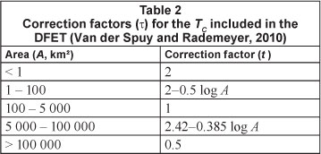
The T_C-based critical storm durations in each catchment under consideration were determined by using Eq. (7), as developed by the United States Bureau of Reclamation (USBR, 1973) and recommended by SANRAL (2006) for use in defined, natural watercourses/channels. In other words, the occurrence of overland flow in the upper reaches of a catchment was also regarded as channel flow; thus taking cognisance of the dominant processes present in the medium to large catchment areas under consideration. Equation (7) is also used as a default in conjunction with the Kerby equation (also available in the DFET for overland flow) to estimate the total travel time for the deterministic flood estimation methods. Van der Spuy and Rademeyer (2010) highlighted that Eq. (7) tends to result in estimates that are either too high or too low and recommended the use of a correction factor (t), which is also included in the DFET and listed in Table 2. Although these proposed correction factors were not scientifically reviewed, similar evidence of the 'poor' translation of runoff volumes into hydrographs and associated peak discharges due to inconsistent catchment response time estimates in ungauged catchments were demonstrated by Smithers et al. (2007).

 

 

where:

The design rainfall information, based on the selected database, method of averaging and DDF relationship, was then used as input to the various design flood estimation methods available in the DFET.

Probabilistic analysis functionalities

In the literature review it was highlighted that a regional approach should be adopted when the observed flood peak data at a single site are insufficient for frequency analysis. In recognition of the practising engineers' possible time and human resource constraints to implementing an extensive regional approach for each new project, 2 single-site approaches were included to assist the user group of the DFET. These two approaches are respectively referred to as the Square Root Area Method (SRAM) and Mean Logarithm Value Approach (MLVA) (Van der Spuy and Rademeyer, 2010). The intended field of application, advantages and inherent limitations associated with the SRAM and MLVA are highlighted in the following paragraphs:

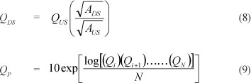
In the SRAM (Eq. (8)), the AMS at single sites either up-or downstream, or from sites in close proximity to the site of interest, could be combined based on the assumption that the temporal and spatial variability of the flood-producing mechanisms in the two or more catchments under consideration are relatively homogeneous (Van der Spuy and Rademeyer, 2010). The SRAM is especially useful to supplement the record length at dams, using data from a flow-gauging station just downstream or upstream from the dam which might have been operational prior the construction of the dam.

The MLVA (Eq. (9)) is based on the combination of the mean values of the logarithms of two or more probability distributions at a single site. Equation (9) could be used to establish the applicability of theoretical probability distributions to specific return-period ranges, e.g., the LP3 fits the lower recurrence interval values better and the GEV the rest. It could also improve design flood estimations based on the AMS at a single site characterised by insufficient record lengths, e.g., missing data, low outliers and flood peaks exceeding the hydraulic capacity of flow-gauging structures. These insufficient record lengths are likely to make it impossible to conclusively select a single probability distribution that could consistently provide flood frequency estimates for return periods much greater than the period of record. Similar sentiments are expressed by Schulze (1989), who argued about the difficulty in fitting a single theoretical probability distribution to a short record length, while Alexander (2012) questioned the accuracy of selecting only a single suitable probability distribution at a particular flow-gauging site.

where:

The individual peak flows (Q_i) in Eq. (9) can either be based on the combination of two or more theoretical probability distributions, e.g., LN, LP3, GEV and/or GLO distributions. The DWA (Directorate: Flood Studies) recommends and uses both of these approaches (Eqs. (8) and (9)) in their flood studies and safety evaluation of dams (Van der Spuy and Rademeyer, 2010). In probabilistic analyses the distribution of the population is estimated from the available observed flood peak data. The best fit of these theoretical probability distributions to the observed flood peak data is then assumed to be the probability distribution representative of the entire population used to estimate the design flood. It could be argued that the MLVA as presented here has no theoretical basis. It is, however, up to the individual practitioner to make that decision and is only included in the DFET to provide some additional support in the decision-making process towards an acceptable peak flood estimate for various probabilities. It could also be argued that a mathematical relationship (e.g., polynomial) fitted to the plotted AMS and return period would be a better alternative to use in such a case.

Subsequently, in order to demonstrate and not promote the use of Eqs. (8) and (9) in the DFET, one or both of these approaches were used where applicable during this study.

Comparison of design flood estimation methods using the DFET

The details of the design flood estimation methods available in the DFET were discussed in the literature review and are listed in Appendix A. Most of the standard design information required by these methods was either incorporated as part of the standard algorithms and/or as 'design tables' in the DFET for easy reference, with the option that automated input can be changed to user-defined input.

In the subsequent sections the use of any specific design flood estimation method associated with a specific areal limitation is not propagated. In order to do a comparison between the probabilistic methods and the suite of deterministic and empirical methods available in the DFET, as well as to investigate the study assumptions, the use of catchment areas exceeding these proposed areal limitations was inevitable.

Probabilistic methods

In cases where observed flood peak data had a sufficiently long record length (N), it was generally accepted that for return periods up to 2N, the probabilistic method results could be regarded as the most reliable estimates. Probabilistic analysis of the AMS was conducted at a representative flow-gauging station in each catchment under consideration to summarise the observed flood peaks, estimate parameters and select appropriate theoretical probability distributions. The observed flood peaks were summarised by ranking the AMS in a descending order of magnitude; a process which is automated in the DFET. The Cunnane plotting position, based on Eq. (1), was used to assign an exceedance probability to the plotted values.

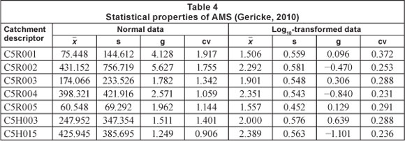
The statistical properties (mean, standard deviation, skew-ness and coefficient of variation) of each AMS (normal and log₁₀-transformed) were calculated by using the DFET, after which the most suitable theoretical probability distribution was selected. Equations (8) and/or (9) were only used in cases where the AMS at a particular flow-gauging site was regarded as insufficient and/or where suitable flow-gauging stations with a high degree of homogeneity were in close proximity.

However, the statistical properties, visual inspection of the plotted values and goodness-of-fit (GOF) statistics, i.e., regression (coefficient of determination) and descriptive (Chi-square) statistics, were used in all cases to select the most suitable single probability or combined probability distribution in Eq. (9). The coefficient of determination (r2) calculations were based on the full record length where the ranked observed values, with their associated probability or return period, were compared with the theoretical probability distributions. The Chi-square statistics were evaluated at a 95% confidence level by making use of the concept of contingency tables (Yount, 2006), which consist of margin totals used to establish the expected estimated values. The margin totals comprise of row and column variables representative of the AMS and theoretical probability distribution values. Thus, for each probability of exceedance, the row totals were calculated as the sum of the AMS and theoretical probability distribution values, while the column totals were based on the sum of all the different individual column variables (e.g. AMS, theoretical probability distribution value and row totals). The expected estimated values were then calculated as the ratio of the product of row and column totals to the grand total, where the grand total either equals the sum of the row or column totals. All the calculations were tested for correctness by ensuring that the sum of the AMS values is equal to the sum of the expected estimated values.

Both the EV1 and LEV1 probability distributions have a fixed skewness of 1.14; hence the limited use thereof in flood hydrology. The LN distribution was only used where the logarithms of the AMS have near symmetrical distribution or where the skewness coefficients were close to zero. In all other asymmetrical data sets, the LP3 distribution was used instead. The GEV distributions were used at asymmetrical data sets characterised by either positive (EV2) or negative (EV3) skewness coefficients.

Deterministic and empirical methods

The developed DFET was used to process all the catchment parameters and design rainfall information to be used as input to the various deterministic and empirical methods, with the remainder of the calculations being fully automated. The standard procedure and techniques associated with each deterministic and empirical method were used by default, while taking cognisance of the assumptions, areal limitations and intended application of each method (refer to Tables A2 and A3, Appendix A). However, since this paper attempts to demonstrate the use and functionality of the DFET, rather than to propose any specific design flood estimation method with specific reference to the study assumptions, most of the catchment areas under consideration exceeded the recommended areal limitations. In essence, these medium to large gauged catchment areas were intentionally selected to merely investigate the study assumptions and to highlight the practising engineers' dilemma, without violating the methods' basic assumptions.

 

Results and discussion

The results based on the methodology used during this study are subsequently discussed.

Development of the DFET

The schematic layout and 'HOME' page of the DFET are shown in Figs. 2 and 3, respectively. The HOME page enables the viewing and/or editing of the contents of relevant databases and design tables, design flood estimation methods, GIS-based maps and graphical plots contained in the various worksheets. It also serves as the primary worksheet with click buttons which activate macros to direct or redirect the user to any required worksheet.

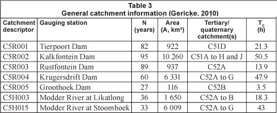
The general catchment information (flow-gauging station number and name, AMS record length (N), catchment area composition and sizes and the T_C) applicable to each of the seven gauged sub-catchments in the study area (C5 secondary drainage region) are listed in Table 3. The catchment areas typically ranged from 116 kitfto 10 260 kmtf, with associated times of concentration ranging between 3.5 h and ± 2 days. A DWA flow-gauging station is situated at the outlet of each of the catchments under consideration. The flow-gauging station numbers were therefore used as the catchment descriptor, for easy reference, in all the tables and figures included in this paper.

 

 

Catchment parameter estimation

An example of the average catchment slope worksheet is illustrated in Fig. 4. The user is only required to enter information in the applicable light-green shaded single cells or cell ranges. In each case, comment boxes, which serve as an 'on-screen help function', are also included. A total of 7 500 horizontal distances between consecutive contours could be entered; however, in this example, only 2 200 grid points were used. The average catchment slope estimation results based on the Neighbourhood (DEM-based), Grid and Empirical methods varied between 2.9% and 4.2% in this particular example (C5R004 catchment). The appropriate option button (DEM or USER INPUT) contained in the group box was selected to indicate the preferential use thereof. The Grid method results used to determine the slope frequency distribution classes are shown in cell range A13: I14.

An example of the average main watercourse slope worksheet and longitudinal profile plot is illustrated in Figs. 5 and 6, respectively. The user is only required to enter the longitudinal profile information in cell range B22: C171, after which the average main watercourse slopes are automatically estimated and plotted on the longitudinal profile. The average main watercourse slope estimation results based on the Equal-area, 10-85 and Taylor-Schwarz methods (Eqs. (4) to (6)) varied between 0.00102 mm^-1 and 0.00131 mm^-1 in this particular example. The appropriate option button (10-85 METHOD) contained in the group box was selected to indicate the preferential use thereof.

Design point rainfall information and estimation methods

Figure 7 is illustrative of the SAWS daily rainfall stations used (not all of the stations are shown) in this particular example. None of the check boxes for 'Outside catchment' in Fig. 7 was selected, since all of the daily rainfall stations selected were within the catchment boundary. However, the check boxes must be selected in cases where the Thiessen Polygon method is also based on daily rainfall stations outside the catchment boundary, but included in the list of rainfall stations. These selections will also have an influence on the Arithmetic Mean method, since this method considers only the stations within the catchment boundary.

The MAP, daily design rainfall information (P_T) and average number of thunder days per year (R), representative of each daily rainfall station as selected in Fig. 7, were automatically obtained from both the RLMA-SAWS and TR102 databases. The averaged MAP, P_T and R values (based on both the Thiessen Polygon and Arithmetic Mean methods) are shown in Fig. 8. A design rainfall group box with option buttons is also included in the DFET to enable the user to select the most appropriate design rainfall database and averaging method.

Figure 9 illustrates the averaged 1' x 1' Grid RLMA&SI design rainfall values as obtained from the design rainfall software developed by Smithers and Schulze (2003). In most of the catchments under consideration, the RMLA&SI approach resulted in the most reliable and consistent design rainfall estimates (Gericke and Du Plessis, 2011).

Probabilistic analyses

The SRAM (Eq. (8)) worksheet is shown in Fig. 10. In this example, the record length of Krugersdrift Dam (C5R004) was extended by using observed flood peaks from a river flow-gauging station (C5H015) just upstream from the dam-site, since the latter was operational prior to the construction of the dam. In other words, the AMS of the river flow-gauging station listed in cell range F14: F36, was used to extend the dam's record length with 23 years, using a square root area factor of 1.026. Similar procedures were used for the other dam flow-gauging stations used in this study.

The MLVA (Eq. (9)) worksheet is shown in Fig. 11. In this example, the check boxes for both the LP3/MM and GLO/LM were ticked to include these two probability distributions in the MLVA, with the results provided in cell range J17 to J26.

Comparison of design flood estimation methods using the DFET

The purpose of this section is to demonstrate the use and functionality of the developed DFET by comparing and assessing the probabilistic, deterministic and empirical flood estimation method results at a single site in the gauged sub-catchments of the study area.

Probabilistic methods

The statistical properties of the AMS used during the probabilistic analyses as listed in Table 4 are characterised by a high degree of variability and skewness typical of the flood peaks in South African rivers. In most of the catchments, due to the high variability, the dispersion about the mean (standard deviation) is relatively high. The skewness coefficients are indicative of the asymmetrical nature of the AMS, while the lower tail of the probability distribution curves was in general longer than the upper tail. The probabilistic design flood estimation results are presented in Table 5. Both the probabilistic design flood estimation results based on the individual theoretical probability distributions and the MLVA (Eq. (9)) are shown. The return periods range from 2 to 200 years, with the chosen single or combined theoretical probability distribution(s) applicable to a specific return period range indicated in the last column of Table 5. In the case of the MLVA, the maximum and minimum return period values used to define the lower (e.g., 2- to 10-year) and higher (e.g., 10- to 200-year) return period ranges, were selected as equal (e.g., 10), to enable a smooth probabilistic plot when Eq. (9) is used. In other words, the theoretical probability estimates at this cross-over point were 'averaged' using both estimates from the lower and higher return period ranges.

 

 

 

 

The coefficients of determination (r²) indicated a high degree of association between the Cunnane plotted AMS values and the theoretical probability distributions, with 0.85 as the poorest correlation. In all the gauged sub-catchments of the study area, except C5R003, C5H003 and C5H018, the Chi-square statistic was less than the limiting critical value and the confidence level larger than the significance level, in other words, the null hypothesis (that the AMS could have been drawn from the theoretical probability distributions evaluated at a 95% confidence level), could be accepted.

The LP3/MM probability distribution was the only distribution which was selected as the most suitable distribution in 43% of the catchments. The MLVA inclusive of the LP3-GEV/MM probability distributions was selected as the most appropriate in 43% of the catchments, followed by the MLVA inclusive of the LP3/MM-GLO/LM probability distributions in 14% of the catchments. The LP3/MM probability distribution fitted the lower recurrence interval values (T < 20 years) the best. These selected single or combined theoretical probability distribution(s) applicable to a specific return period range are summarised in the last column of Table 5 and highlight the overall non-homogeneity of the study area in terms of hydro-logical responses and flood statistics.

In recognising the limitations of single-site analyses as opposed to a regional approach, the MLVA is however regarded as not being able to take cognisance of the strong evidence that in South Africa most of the high flood peaks are a result of rare and severe meteorological phenomena. Alexander (2012) also confirmed that the AMS of these floods could consist of a mixture of two or more statistical populations with different parameter values and associated flood peak frequency relationships, particularly if preceding severe rainfall storms occur in close succession. In such a case, the use of the Two-Component Extreme Value (TCEV) distribution as part of a regional approach is suggested. The TCEV could then be used to separate the AMS into 2 statistical populations, e.g., the basic component (more frequent and less intense) and the outlying component (less frequent and more intense) in order to analyse them independently (Fiorentino et al., 1985).

The probability plots based on the results contained in Table 5 are shown in Figs. 12 to 18. Figures 14 and 17 are illustrative of AMS typically containing 2 distinct statistical populations, e.g., the basic component (T . 10 years) and the outlying component (T.>.10.years).

 

 

 

 

 

 

 

 

 

 

 

 

Deterministic and empirical methods

Table 6 provides a summary of the GOF statistics for the design flood estimation results (Q_D), based on the deterministic and empirical methods, compared to the MLVA (Q_P) for return periods ranging from 2 to 200 years. The Root Mean Square Error (RMSE), r2 values and Q_D/Q_P average ratios listed in the table represent the catchment values associated with a specific method, for all of the return periods under consideration. The RMSE was specifically included to ensure that the accumulated over- and/or underestimations are accounted for, i.e., to highlight the actual size (not source or type) of errors produced by a specific method, with the objective function to minimise the RMSE to zero.

The results contained in Table 6 were indicative of several trends associated with specific areal ranges and return periods, which are highlighted in the following paragraphs:

Areal range (100 km² < A < 500 km²):

• C5R005 (116 km²): All the deterministically estimated flood peaks, except for the SUH and LRH methods, exceeded the MLVA values. On average, the overestima-tion ranged from +39% to +48%, with this tendency quite evident in the lower recurrence intervals (e.g., 2 to 10 years). The SCS method demonstrated the best average results, with an RMSE value of 61, r2 value of 0.98 and an associated average overestimation of +41%. It could be argued that the SUH method demonstrated equally accurate results, with an RMSE value of 71 and an underestimation of only -6%. The empirically estimated flood peaks (MIPI and CAPA methods) were characterised by average under-estimations ranging between -14% and -39%. The MIPI method had the lowest RMSE value (59), but was only used to estimate the 10-year to 100-year flood peaks; in other words, only 57% of the sample range. Subsequently, the GOF statistics might be misleading. The poorest average results were demonstrated by the CAPA method (RMSE = 162, r2 = 0.99, -39% underestimation), which is likely due to the magnitude of underestimations throughout all the return periods.

Areal range (500 km2 < A < 1 000 km2):

• C5R001 (922 km2): All the deterministically and empirically estimated flood peaks, except for the CAPA method, exceeded the MLVA values. On average, the overestima-tion varied between +12% and +62%. The best average results were demonstrated by the LRH method (RMSE = 116, r2 = 0.99, +26% overestimation), followed by the RM (RMSE = 121, r2 = 0.99, +15% overestimation). The poorest average results were demonstrated by the ARM (RMSE = 188, r2 = 0.99 and +12% overestimation). All the methods demonstrated a tendency to overestimate the lower recurrence intervals (e.g. 2 to 10 years) by a larger factor, with individual Q_D/Q_P ratios ranging between 1.5 and 3.5.

• C5R003 (937 km2): On average, only the SCS and SDF methods exceeded the MLVA values, with overestima-tions in the order of +20%. The SCS method demonstrated the best average results, i.e., RMSE = 97, r2 = 0.99 and +19% overestimation, followed by the LRH method (RMSE = 108, r2 = 0.95 and -2% underestimation). The poorest average results were demonstrated by the SDF (RMSE = 210, r2 = 0.98 and +22% overestimation) and CAPA (RMSE = 190, r2 = 0.98 and -22% underestimation) methods.

Areal range (1 000 km2 < A < 5 000 km2):

• C5H003 (1 650 krtf): Similar trends as identified at C5R003 characterised the results. However, on average, the over-and underestimations slightly decreased and increased, respectively.

Areal range (5 000 km2 < A < 10 500 km2):

• C5H015 (6 009 km2): Only the SDF method exceeded the MLVA values and also demonstrated the poorest results, i.e., RMSE = 997, r² = 0.93 and +36% overestimation. The best average results were demonstrated by the SCS method (RMSE = 169, r2 = 0.96 and -11% underestimation), followed by the CAPA method (RMSE = 274, r2 = 0.93 and -12% underestimation).

• C5R004 (6 331 km2): Similar trends as identified at C5H015 characterised the results. However, on average, the over- and underestimations slightly decreased and increased, respectively, while the best average results were demonstrated by the CAPA method (RMSE = 355, r2 = 0.99 and -21% underestimation). The poorest average results were demonstrated by the ARM with the RMSE = 691, r2 = 0.99 and -31°% underestimation.

• C5R002 (10 260 km2): On average, only the SCS and SDF methods exceeded the MLVA values, with +4% and +52%, respectively. The best average results were demonstrated by the SCS method with the RMSE = 762, r2 = 0.99 and +4% " overestimation. The poorest average results were demonstrated by the SUH (RMSE = 1 275, r2 = 0.99 and -45% underestimation) and LRH (RMSE = 1 232, r2 = 0.99 and -43% underestimation) methods.

In order to enhance the understanding of the results discussed above, it was decided to make use of a scoring rubric to enable the ranking of each method in the 4 different areal ranges. The use of average Q_D/Q_P ratios might be misleading; therefore only the RMSE was used in the scoring rubric to account for the accumulated over- and underestimations. Since 7 methods (excluding the MIPI method; refer to reasons provided above) were used in the comparisons, a scoring scale of 1 to 7 (with 1 = lowest RMSE and 7 = highest RMSE) was implemented. The results are summarised in Table 7, while Fig. 19 provides a visual measure of performance showing the RMSE based on the results contained in Table 6.

 

 

Based on above-listed results (Tables 6, 7 and Fig. 19), the following aspects were interesting to note: • All the deterministic methods tend to overestimate the lower recurrence interval floods (T < 10 years) more frequently, with Qj/Q_P ratios up to 2.8 in all the areal ranges.

• In contrast, the empirical methods (e.g., MIPI and CAPA) underestimated all the MLVA values for all recurrence intervals and areal ranges, except for the 2- and 5-year recurrence intervals in some of the catchments (e.g., C5R001). The fact that empirical methods are less reliant on design rainfall information and catchment response time than deterministic methods may have contributed to this trend. In essence, this highlights the presence of subjectivity in using different (outdated) DDF relationships in conjunction with certain deterministic flood estimation methods as stipulated in the SANRAL (2006) Drainage Manual. The poor overall ranking of the ARM (Table 7) is most likely a result thereof. Despite the inclusion of all these 'outdated' DDF methodologies in the DFET, except for the RLMA&SI approach, none of them are proposed for future use in South Africa. However, it is important to note that the DFET was purposely developed to include all recognised estimation methods currently used in South African flood hydrology.

• In most cases the simplified 'small catchment' (A < 15 kitf) deterministic flood estimation methods (e.g. SCS and RM), which were applied far beyond their recommended areal limitations, provided the most acceptable results when compared to the probabilistic analyses applicable to all the return periods, except for the 2-year return period. Based on only the RMSE statistics, the SCS method and RM were also ranked as the best performing methods.

• The deterministic (e.g. SDF, SUH and LRH) methods which are regarded as more applicable to 'medium' (15 km2 < A < 5 000 kitf) and 'large' (A > 5 000 kitf) catchments, demonstrated less acceptable results compared to the 'small catchment' methods, especially in the 'large' catchments. Typically, these methods were ranked between 4^th and last in the range, A > 5 000 km2.

• The LRH method, which is regarded by many practising hydrologists as the 'poorer twin-brother' of the SUH method, proved to be equally reliable compared to the SUH method, especially in the range, 500 < A

< 10 500 km². However, it is important to note that the latter two methods are not independent; subsequently the LRH method cannot be used as an independent check of the more time-consuming SUH method. The fact that the LRH method could be used in catchment areas up to 10 000 km2 (Bauer and Midgley, 1974) may have contributed to this trend, although the use of Muskingum routing parameters based on the proportionality ratio of TL = 0.6T_C (Van der Spuy and Rademeyer, 2010) is more likely to be responsible for these slight differences. Concurrently, the following question can also be raised: 'Why limit the areal application of the SUH method only to 5 000 knr⁵, if catchment areas up to 22 163 km2 were used during the development thereof?'

• Apart from all the probabilistic and empirical methods, the SDF method is regarded as the only deterministic method suitable to use in catchment areas up to 40 000 km2

(Alexander, 2002), while SANRAL (2006) specify no areal limitation for this method. Ironically, some of the poorest results were demonstrated by the SDF method, with average catchment-specific overestimations ranging from 20% to 62%, while some individual return periods were overestimated by 110%. Despite these results, the SDF method proved to be more reliant in medium/larger catchment areas than in small catchment areas, hence its overall 4^th ranking (c.f. Table 7).

 

Conclusions and recommendations

The developed DFET presented in this paper provides designers with an easy-to-use software tool for the rapid estimation and evaluation of alternative design flood estimation methods currently available in South Africa for applications at a site-specific scale in both gauged/ungauged and small/large catchments. The DFET was provided to a variety of participating engineers at Continuous Professional Development (CPD)-accredited flood hydrology courses arranged by the University of Stellenbosch on bi-annual basis. This resulted in constructive feedback, i.e., different practitioners/users played a pivotal role in the validation of the DFET code by means of comparisons using either hand-calculations or other relevant software, which was incorporated into the final version of the DFET. The focus user group for the developed DFET will comprise of general civil engineering technicians, engineering technologists and engineers employed at consultancies, who are not necessarily specialists in the field of flood hydrology who would be more likely to follow a regional approach.

The design flood estimation results based on the probabilistic, deterministic and empirical methods available in the DFET highlighted the following aspects:

• The LP3 and GEV theoretical probability distributions using the Cunnane plotting formula proved to be most suitable for probabilistic design flood estimation in the C5 secondary drainage region of South Africa (c.f. Table 5).

• The SRAM (Eq. (8)), within the limitations of regional homogeneity, could be used to improve the probabilistic design flood estimations at a single site in gauged catchments which are regarded as homogeneous. However, the fact that the 'appropriateness' of different theoretical probability distributions varied from site to site, as well as the highly variable rainfall characterising the C5 secondary drainage region, emphasised that the use thereof must be carefully considered.

• The MLVA (Eq. (9)) must only be used to optimise the graphical fitting of theoretical probability distributions. This will enable users to make more informed decisions about which individual theoretical probability distribution to use. The MLVA is also regarded as not being able to take cognisance of the presence of two or more statistical populations present in observed flood peak data. Arguably, fitting a relationship either manually or mathematically to the plotted AMS and return period may be preferable to the MLVA approach.

• The use of the TCEV theoretical distribution as part of a regional approach must be further investigated to analyse the AMS characterised by multiple statistical populations.

• An important aspect is the need for consistency when deterministic flood estimation methods are used. By using the RLMA&SI approach as the 'only' DDF relationship applicable to all design flood estimation methods, consistency in terms of design rainfall could be achieved. However, considerable inconsistency remains in the estimation of the catchment response time which impacts on the estimated design rainfall intensity and associated runoff (Smithers, 2012).

• The overall ranking of the deterministic flood estimation methods based on the RMSE statistics in the four different areal ranges confirmed that the SCS method is the most appropriate method, followed by the RM and LRH method. Despite these results, potential users of the DFET are urged to take cognisance of each method's basic assumptions, methodological approaches and limitations, in order to ensure that the intended use of a method is not violated.

• The poor overall ranking (6^th) of the empirical methods highlighted the non-homogeneity of the study area, while it reiterated the importance of limiting the application of empirical methods to their homogeneous catchments or regions of original development. However, the empirical methods proved to be the most appropriate in catchment areas larger than 5 000 km2.

• It is also important to note that all methods used to describe natural events (e.g. rainfall and floods) are to some extent empirically-based, i.e., contingent and revisable. The need for revision arises if the estimation results are consistently refuted by actual observations, which was the case in this study. Subsequently, the updating of existing methods and/ or development of new methods is not negotiable.

All these results emphasised that there is no single design flood estimation method that is superior to all other methods used to address the wide variety of flood magnitude-frequency problems that are encountered in practice. Practising engineers' still have to apply their own experience and knowledge to these particular problems until the search for universally applicable design flood methods in South Africa produces methods by which to overcome all the inherent uncertainties present in flood hydrology. In other words, the question is not about 'which method (recognising each method's inherent limitations or assumptions) to use when (gauged or ungauged catchments), where (urban vs. rural areas with an associated areal limitation) and how (single site vs. regional approach)', but rather 'what are we going to do about the practising engineers' dilemma?'

The answer to this question is very simple, but more difficult to facilitate: The gap between flood research and practice in South Africa can only be narrowed by improving and updating existing (outdated) design flood estimation methods and/ or evaluating methods used internationally and developing new methods for application in South Africa. However, to facilitate this, the establishment of a flood hydrology research unit, similar to the Hydrological Research Unit (HRU) at the University of the Witwatersrand in the 1970s, and sufficient funding (e.g. from DWA and WRC) are required.

 

References

ADAMSON PT (1981) Southern African Storm Rainfall. Technical Report TR102. Department of Environment Affairs and Tourism, Pretoria.         [ Links ]

ALEXANDER WJR (1990) Flood Hydrology for Southern Africa.         [ Links ]

SANCOLD, Pretoria. ALEXANDER WJR (2001) Flood Risk Reduction Measures: Incorporating Flood Hydrology for Southern Africa. Department of Civil and Biosystems Engineering, University of Pretoria, Pretoria.         [ Links ]

ALEXANDER WJR (2002) The Standard Design Flood. J. S. Afr. Inst. Civ. Eng. 44 (1) 26-30.         [ Links ]

ALEXANDER WJR (2012) Personal communication, 17 February 2012. Professor Emeritus, University of Pretoria, Pretoria.         [ Links ]

BAUER SW and MIDGLEY DC (1974) A Simple Procedure for Synthesizing Direct Runoff Hydrographs. Hydrological Research Unit, University of Witwatersrand, Johannesburg.         [ Links ]

BEVEN KJ (2000) Rainfall-Runoff Modelling: The Primer. John Wiley & Sons, Chichester.         [ Links ]

CHADWICK AJ and MORFETT JC (2004) Hydraulics in Civil and Environmental Engineering (4^th edn.) E & FN Spon, Chapman and Hall, London.         [ Links ]

CHOW VT, MAIDMENT DR and MAYS LW (1988) Applied Hydrology. McGraw-Hill, New York.         [ Links ]

CSIR (COUNCIL FOR SCIENTIFIC AND INDUSTRIAL RESEARCH) (2001) GIS Data: Classified Raster Data for National Coverage based on 31 Land Cover Types. National Land Cover Database. Environmentek, CSIR, Pretoria.         [ Links ]

CULLIS J, GORGENS AHM and LYONS S (2007) Updated Guidelines and Design Flood Hydrology Techniques for Dam Safety. WRC Report No. 1420/1/07. Water Research Commission, Pretoria.         [ Links ]

CUNNANE C (1978) Unbiased plotting positions - A review. J. Hydrol. 37 205-222.         [ Links ]

DWAF (DEPARTMENT OF WATER AFFAIRS AND FORESTRY, SOUTH AFRICA) (1995) GIS Data: Drainage Regions of South Africa. Department of Water Affairs and Forestry, Pretoria.         [ Links ]

ESRI (ENVIRONMENTAL SYSTEMS RESEARCH INSTITUTE) (2006) ArcGIS Desktop Help: Spatial Analyst Slope Algorithm. Environmental Systems Research Institute, Redlands, California.         [ Links ]

FIORENTINO M, VERSACE P and ROSSI F (1985) Regional flood frequency estimation using the TCEV distribution. Hydrol. Sci. J. 30 (3) 51-64.         [ Links ]

FRANCOU J and RODIER JA (1967) Essai de classification des crues maximales. In: Proc. Leningrad Symposium on Floods and their Computation, UNESCO, August 1967.         [ Links ]

GERICKE OJ (2010) Evaluation of the SDF Method using a customised Design Flood Estimation Tool. Unpublished M.Sc. Eng. Dissertation, Department of Civil Engineering, Stellenbosch University, Stellenbosch.         [ Links ]

GERICKE OJ and DU PLESSIS (2011) Evaluation of critical storm duration rainfall estimates used in flood hydrology in South Africa. Water SA 37 (4) 453-470.         [ Links ]

GORGENS AHM (2002) Design flood hydrology. In: Basson G (ed.) Proc. Design and Rehabilitation of Dams. Institute for Water and Environmental Engineering, Department of Civil Engineering, Stellenbosch University. 460-524.         [ Links ]

GORGENS AHM (2007) Joint Peak-Volume (JPV) Design Flood Hydrographs for South Africa. WRC Report No. 1420/3/07. Water Research Commission, Pretoria.         [ Links ]

GUPTA RD and KUNDU D (2007) Generalised exponential distribution: existing methods and recent developments. J. Stat. Plann. Inference 137 (11) 3537-3547.         [ Links ]

HRU (HYDROLOGICAL RESEARCH UNIT) (1972) Design Flood Determination in South Africa. HRU Report No. 1/72. Hydrological Research Unit, University of the Witwatersrand, Johannesburg.         [ Links ]

IH (INSTITUTE OF HYDROLOGY) (1999) Flood Estimation Handbook. Institute of Hydrology, Wallingford, Oxfordshire.         [ Links ]

KITE GW (1988) Frequency and Risk Analysis in Hydrology (Revised edn.). Water Resources Publications, Littleton, Colorado.         [ Links ]

KJELDSEN TR and JONES DA (2004) Sampling variance of flood quantiles from the generalised logistic distribution estimated using the method of L-Moments. Hydrol. Earth Syst. Sci. 8 183-190.         [ Links ]

KOVÁCS ZP (1988) Regional Maximum Flood Peaks in South Africa. Technical Report TR137. Department of Water Affairs, Pretoria.         [ Links ]

LYNCH, SD (2004) Development of a Raster Database of Annual, Monthly and Daily Rainfall for Southern Africa. WRC Report No. 1156/1/04. Water Research Commission, Pretoria.         [ Links ]

MADSEN H, PEARSON CP and ROSBJERG D (1997) Comparison of annual maximum series and partial duration series methods for modelling extreme hydrologic events. Water Resour. Res. 33 759-769.         [ Links ]

McCUEN RH (2005) Hydrologic Analysis and Design (3^rd edn.). Prentice-Hall, Upper Saddle River, New York.         [ Links ]

McPHERSON DR (1983) Comparison of mean annual flood peaks calculated by various methods. In: Maaren H (ed.) Proc. South African National Hydrology Symposium. Technical Report TR119, Department of Environmental Affairs and Tourism, Pretoria. 236-250.         [ Links ]

MIDGLEY DC and PITMAN WV (1978) A Depth-Duration-Frequency Diagram for Point Rainfall in Southern Africa. HRU Report No. 2/78. Hydrological Research Unit, University of the Witwatersrand, Johannesburg.         [ Links ]

MIDGLEY DC, PITMAN WV and MIDDLETON BJ (1994) Surface Water Resources of South Africa. Volume 2, Drainage Region C, Vaal: Appendices. WRC Report No. 298/2.1/94. Water Research Commission, Pretoria.         [ Links ]

PARAK M and PEGRAM GGS (2006) Rational formula from Runhydrograph. Water SA 32 (2) 163-180.         [ Links ]

PITMAN WV and MIDGLEY DC (1967) Flood studies in South Africa: Frequency analysis of peak discharges. Trans. S. Afr. Inst. Civ. Eng. August 1967.         [ Links ]

PITMAN WV and MIDGLEY DC (1971) Amendments to Design Flood Manual HRU 4/69. HRU Report No. 1/71. Hydrological Research Unit, University of the Witwatersrand, Johannesburg.         [ Links ]

PEGRAM GGS (2003) Rainfall, rational formula and regional maximum flood: Some scaling links. Keynote Paper. Aust. J. Water Resour. 7 (1) 29-39.         [ Links ]

PEGRAM GGS and PARAK M (2004) A review of the Regional Maximum Flood and Rational Formula using geomorphological information and observed floods. Water SA 30 (3) 377-392.         [ Links ]

PILGRIM DH and CORDERY I (1993) Flood runoff. In: Maidment DR (ed.) Handbook of Hydrology. McGraw-Hill, New York.         [ Links ]

RAHMAN A, WEINMANN PE, HOANG TMT and LAURENSON EM (2002) Monte Carlo simulation of flood frequency curves from rainfall. J. Hydrol. 256 196-210.         [ Links ]

REICH BM (1963) Short-duration rainfall-intensity estimates and other design aids for regions of sparse data. J. Hydrol. 1 3-28.         [ Links ]

SANRAL (SOUTH AFRICAN NATIONAL ROADS AGENCY LIMITED) (2006) Drainage Manual (5^th edn.). South African National Roads Agency Limited, Pretoria.         [ Links ]

SCHULZE RE (1989) Non-stationary catchment responses and other problems in determining flood series: A case for a simulation modelling approach. In: Proc. 4^th SANCIAHS National Hydrological Symposium, 20-22 November 1989, Pretoria. 135-157.         [ Links ]

SCHULZE RE (1995) Hydrology and Agrohydrology: A Text to Accompany the ACRU 3.00 Agrohydrological Modelling System. WRC Report No. TT 69/95. Water Research Commission, Pretoria.         [ Links ]

SCHULZE RE, SCHMIDT EJ and SMITHERS JC (1992) SCS-SA User Manual: PC-Based SCS Design Flood Estimates for Small Catchments in Southern Africa. ACRU Report 40. Agricultural Catchments Research Unit, Department of Agricultural Engineering, University of Natal, Pietermaritzburg.         [ Links ]

SMITHERS JC (2012) Review: Methods for design flood estimation in South Africa. Water SA 38 (4) 633-646.         [ Links ]

SMITHERS JC, CHETTY KT, FREZGHI MS, KNOESEN DM and TEWOLDE MH (2007) Development and Assessment of a Continuous Simulation Modelling System for Design Flood Estimation. WRC Report No. 1318/1/07. Water Research Commission, Pretoria.         [ Links ]

SMITHERS JC and SCHULZE RE (2000a) Development and Evaluation of Techniques for Estimating Short Duration Design Rainfall in South Africa. WRC Report No. 681/1/00. Water Research Commission, Pretoria.         [ Links ]

SMITHERS JC and SCHULZE RE (2000b) Long Duration Design Rainfall Estimates for South Africa. WRC Report No. 811/1/00. Water Research Commission, Pretoria.         [ Links ]

SMITHERS JC and SCHULZE RE (2003) Design Rainfall and Flood Estimation in South Africa. WRC Report No. 1060/01/03. Water Research Commission, Pretoria.         [ Links ]

SMITHERS JC and SCHULZE RE (2004) The estimation of design rainfall for South Africa using a regional scale invariant approach. Water SA 30 (4) 435-444.         [ Links ]

STEDINGER JR, VOGEL RM and FOUFOULA-GEORGIOU E (1993) Frequency analysis of extreme events. In: Maidment DR (ed.) Handbook of Hydrology. McGraw-Hill, New York.         [ Links ]

USBR (UNITED STATES BUREAU OF RECLAMATION) (1973) Design of Small Dams (2^nd edn.). Water Resources Technical Publication, Washington, DC.         [ Links ]

USGS (UNITED STATES GEOLOGICAL SURVEY) (2002) SRTM Topography. URL: http://dds.cr.usgs.gov/srtm/version2_1/Documentation/SRTMTopo.pdf (Accessed 2 June 2010).         [ Links ]

VAN BLADEREN D (2005) Verification of the proposed Standard Design Flood (SDF). SRK Consulting Engineers and Scientists. Report No. 344512/1. Pretoria.         [ Links ]

VAN DER SPUY D and RADEMEYER PF (2010) Flood Frequency Estimation Methods as Applied in the Department of Water Affairs. Department of Water Affairs, Pretoria.         [ Links ]

VAN DIJK M (2005) Utility Programs for Drainage (UPD). Sinotech CC, Pretoria, RSA. URL: http://www.sinotechcc.co.za/Software/UPD/ (Accessed 15 March 2012).         [ Links ]

YEVJEVICH V (1982) Probability and Statistics in Hydrology (1^st edn.). Water Resources Publications, Littleton, Colorado. YOUNT WR (2006) Research Design and Statistical Analysis in Christian Ministry (4^th edn.). Southwestern Baptist Theological Seminary. Fort Worth, Texas.         [ Links ]

 

 

Received 7March 2011;
Accepted in revised form 7 January 2013.

 

 

* To whom all correspondence should be addressed. ffi +2751-507 3516; fax: +2751-507 3254; e-mail: jgericke@cut.ac.za
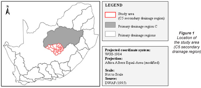
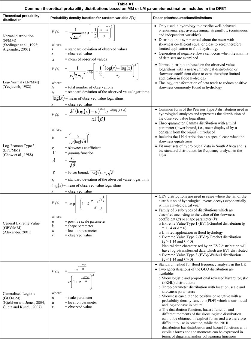
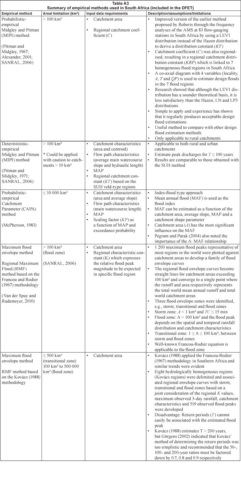
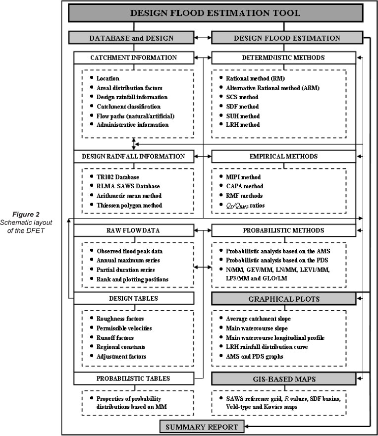
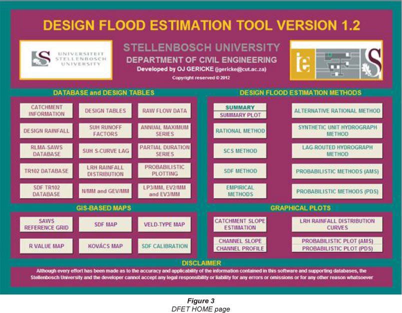
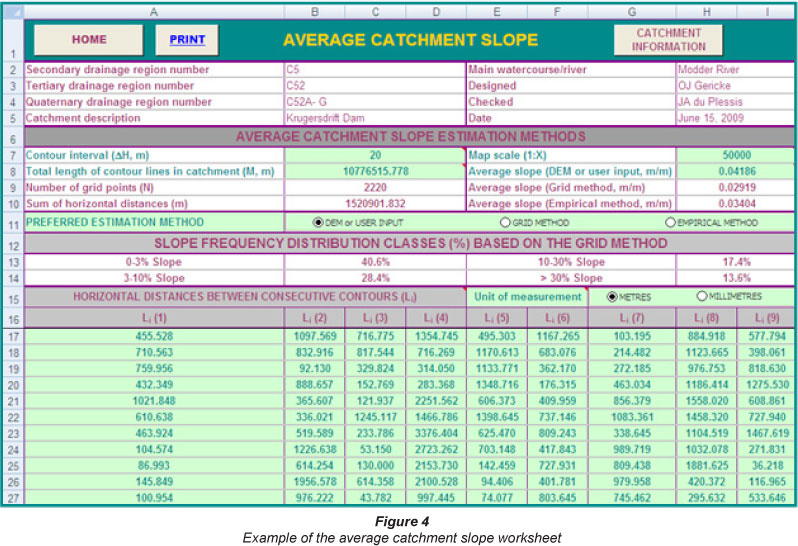
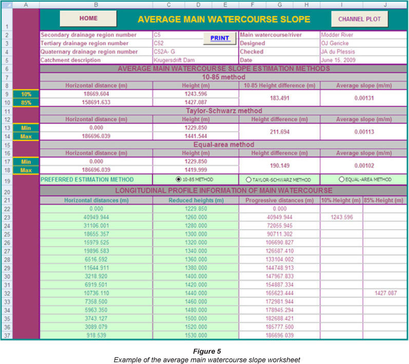
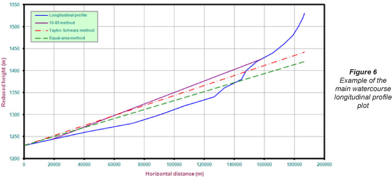
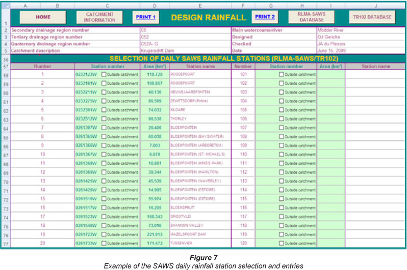
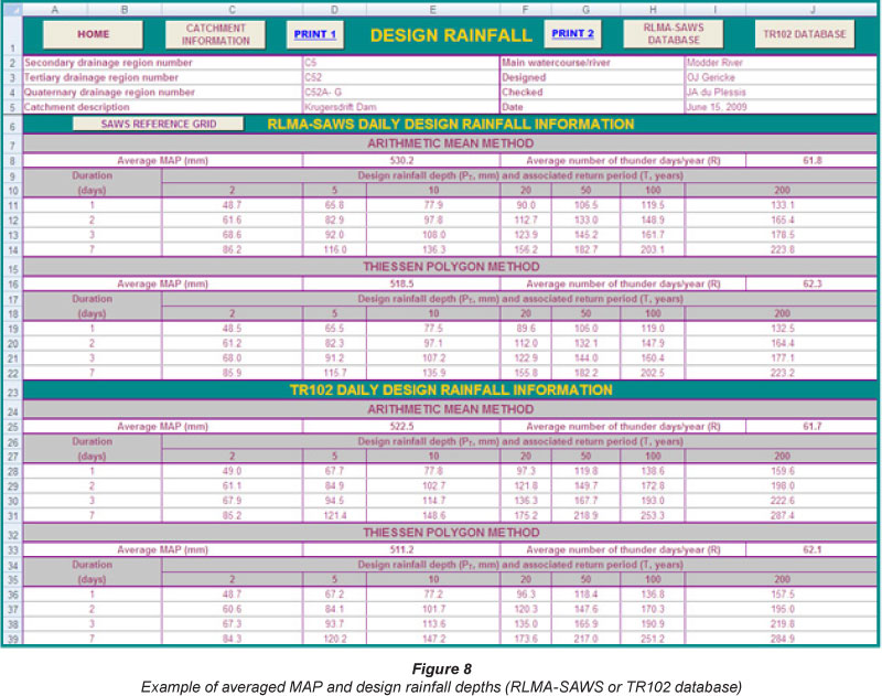
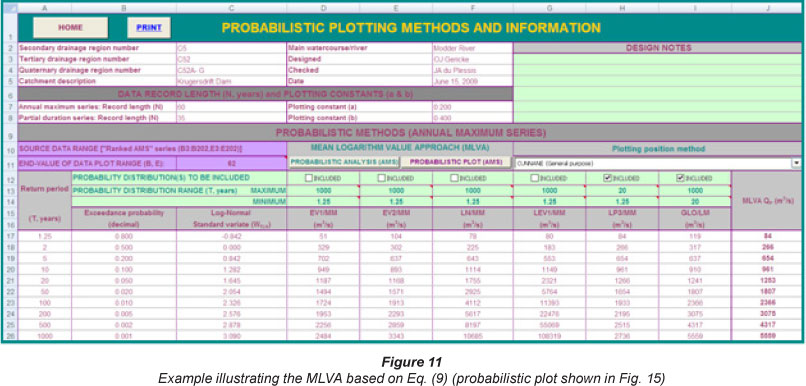
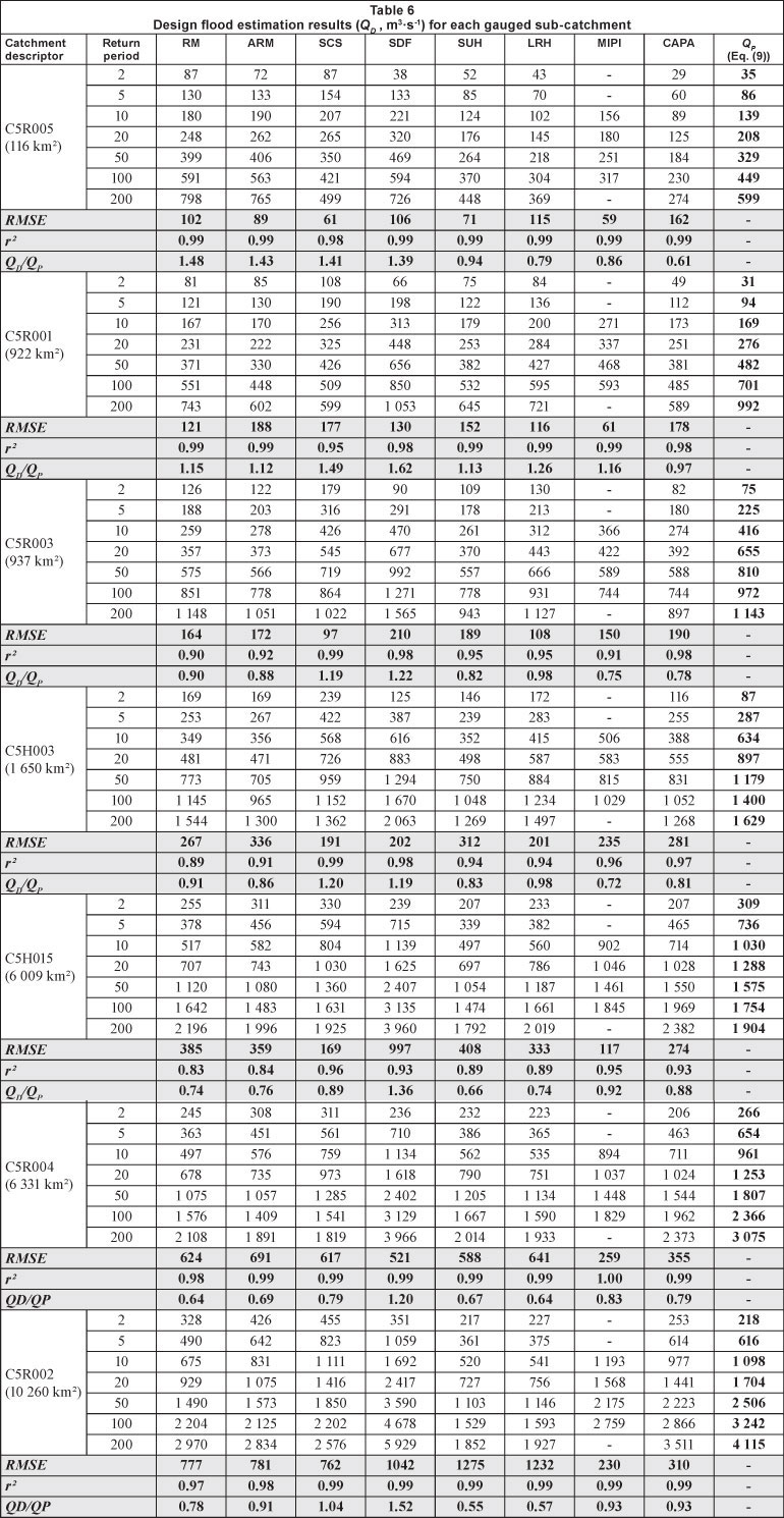