


Services on Demand
Article
 English (pdf)
 Article in xml format
 Article references
Indicators

Related links
-
 Cited by Google
 -
 Similars in Google
Share

 Permalink
Water SA
On-line version ISSN 1816-7950
Print version ISSN 0378-4738
Water SA vol.38 n.5 Pretoria Jan. 2012
A short-range weather prediction system for South Africa based on a multi-model approach
Stephanie LandmanI, II, *; Francois A EngelbrechtIII, IV; Christien J EngelbrechtV; Liesl L DysonII; Willem A LandmanII, III
ISouth African Weather Service, Pretoria 0001, South Africa
IIDepartment of Geography. Geoinformatics and Meteorology, University of Pretoria 0002, South Africa
IIICSIR Natural Resources and the Environment: Climate Studies, Modelling and Environmental Health, Pretoria 0001, South Africa
IVClimatology Research Group, GAES, University of the Witwatersrand, South Africa
VAgricultural Research Council - Institute for Soil, Climate and Water, Pretoria 0001, South Africa
ABSTRACT
The accurate prediction of rainfall events, in terms of their timing, location and rainfall depth, is important to a wide range of social and economic applications. At many operational weather prediction centres, as is also the case at the South African Weather Service, forecasters use deterministic model outputs as guidance to produce subjective probabilistic rainfall forecasts. The aim of this research was to determine the skill of a new objective multi-model, multi-institute probabilistic ensemble forecast system for South Africa. Such forecasts are obtained by combining the rainfall forecasts of 2 operational high-resolution regional atmospheric models in South Africa. The first model is the Unified Model (UM), which is operational at the South African Weather Service. The UM contributes 3 ensemble members, each with a different physics scheme, data assimilation techniques and horizontal resolution. The second model is the Conformal-Cubic Atmospheric Model (CCAM) which is operational at the Council for Scientific and Industrial Research, which in turn contributed 2 members to the ensemble system based on different horizontal resolutions. A single-model ensemble forecast, with each of the ensemble members having equal weights, was constructed for the UM and CCAM models, respectively. These UM and CCAM single-model ensemble predictions are then combined into a multi-model ensemble prediction, using simple un-weighted averaging. The probabilistic forecasts produced by the single-model system as well as the multi-model system have been tested against observed rainfall data over 3 austral summer 6-month periods from 2006/07 to 2008/09, using the Brier skill score, relative operating characteristics, and the reliability diagram. The forecast system was found to be more skilful than the persistence forecast. Moreover, the system outscores the forecast skill of the individual models.
Keywords: short-range, ensemble, forecasting, precipitation, multi-model, verification
Introduction
Precipitation forecasts are of high relevance to users of meteorological information in South Africa, but precipitation is also highly variable in time and space, making it one of the most difficult meteorological variables to predict skilfully. Nonetheless, skilful precipitation forecasts are essential to provide early warning of heavy rainfall and floods that may lead to loss of life and property. Most modern operational weather centres rely on limited-area numerical weather prediction (NWP) models in order to generate reliable and accurate weather forecasts (Stensrud et al., 1999; Toth et al., 2001). At short-range time scales (from 12 h up to 3 days), predicting the location of a precipitation event has a greater error than the prediction of the pattern and amount of precipitation (Theis et al., 2005). The large spatial and temporal variability in rainfall, together with some NWP model errors, contributes to the uncertainties and low skill associated with rainfall predictions (Ebert, 2001; Theis et al., 2005; Roy Bhowmik and Durai, 2010).
Precipitation forecasts from NWP models are often provided in a deterministic manner. An inherent characteristic of deterministic forecasts is that the future state of the atmospher is assumed to be conditional on the present state of the atmosphere only, and evolution of the future state is governed by deterministic equations. Therefore, an accurate short-range numerical forecast is dependent on accurately describing the initial conditions (Kalnay, 2003). The reason for this dependency on accurate initial conditions stems from the chaotic and non-periodic characteristics of the atmosphere (Lorenz, 1963). Forecasts that are initialised with only slightly different initial states progressively diverge as a function of model integration time. Deterministic or best-guess forecasts are therefore considered to be less reliable as the model integration-time increases, due to uncertainties that exist in the initial conditions as well as the internal error (physics and dynamics) of the numerical model itself (Lorenz, 1963; Ebert, 2001; Stensrud et al., 2005; Theis et al., 2005).
Many national meteorological services (NMS) issue precipitation forecasts in terms of subjective probabilities, whereby it is assumed that the user receives additional information regarding the uncertainty pertaining to the specific forecast (Staël von Holstein, 1971). Forecasters have long been aware of the fact that different models often produce a variety of the predicted weather outcomes (Ebert, 2001). The probability forecasts issued by forecasters are subjective because they are based on the forecaster's own insights and experience being used in the mental integration of several model realisations (Staël von Holstein, 1971). Methods that could produce objective probability forecasts at the short-range time-scale have the potential to objectively address, to some extent, the uncertainties associated with describing the initial state of the atmosphere as well as the uncertainties induced by internal model errors (Theis et al., 2005).
An ensemble prediction system (EPS) represents a stochastic approach which couples probability with determinism (Lewis, 2005), and which has the specific aim of predicting the probability of future weather events occurring, in turn addressing the uncertainty of a deterministic forecast (Stensrud et al., 1999). Theis et al. (2005) concluded that precipitation forecasts should be addressed in a probabilistic manner in order to account for the chaotic nature of NWP forecasts. An important goal of ensemble prediction is to provide estimations of the reliability of the forecast being made (Kalnay, 2003; Grimit and Mass, 2005). The ensemble of forecasts from single or multiple numerical weather prediction models provides detail of the forecast, regarding the confidence, possible errors and probability outcomes (Bakhshaii and Stull, 2009).
Ensemble forecasts may be constructed in various ways (e.g. Kalnay, 2003). The traditional approach is to perform multiple model runs using the same model, by initialising each run from initial conditions constructed in a different manner. Single-model ensemble systems effectively inhibit the description of the forecast uncertainty associated with model error, and this may lead to underestimation of the forecast error (Clark et al., 2008). However, multi-model ensemble forecasts better address both the uncertainties that exist in the systematic errors of each numerical model, as well as the uncertainties within the initial conditions (Ebert, 2001). Clark et al. (2008) noted that, in addition to addressing uncertainties in initial conditions, ensemble forecasting, and more specifically multi-model systems, will also inadvertently address errors related to lateral boundary conditions. At the short-range time-scale, synoptic and mesoscale features are less predictable, due to their more chaotic features, than features at the planetary scale (Hamill and Colucci, 1997; Friederichs and Hense, 2008; Roy Bhowmik and Durai, 2010). For this reason, ensemble methods will primarily improve the description of the uncertainty and model error that exists in relation to these shorter-length time-scale features. The model uncertainty can be accounted for by running the same model with different physical parameterisations or analysis times or by using model runs from different numerical models (Bowler et al., 2008b, Wandishin et al. , 2001). Typically, the errors and uncertainties in each individual member of the ensemble cancel out when calculating the ensemble average, making the ensemble average appear relatively smooth (Bowler et al., 2008b; Kalnay, 2003). A multi-model system based on a multi-institute ensemble has the advantage of effectively sharing the computational power needed to construct large ensembles amongst different institutions.
Even though research has shown that an ensemble mean forecast generally outperforms a single deterministic forecast (Ebert, 2001), operational use of short-range ensemble systems has lagged behind that of long-range and medium-range forecasting (Eckel and Mass, 2005). However, there are a number of NMSs that use short-range ensemble prediction systems operationally or quasi-operationally. These include NCEP (USA), INM (Spain), NMI (Norway), the Met Office (UK), DWD (Germany), BoM (Australia) and recently also SAWS (South Africa).
The objectives of this study were to investigate the skill of a South African multi-model ensemble in predicting 24-hour precipitation for South Africa, and to compare the skill of the multi-model ensemble to that of the single-model ensemble systems it is based upon.
In the next section, the observed data sets and forecasting systems are discussed. The construction of the new multi-model ensemble system based on 2 operational NWP models in South Africa and the forecast verification methods applied to describe the accuracy and skill of the system are described in the 'Methods' section. Verification results are presented in the 'Results' section, and conclusions are drawn in the 'Discussion and conclusions' section.
Data
Model data
Unified Model
The Unified Model (UM) is a non-hydrostatic model developed at the UK Met Office (Davies et al., 2005). Its vertical coordinate is based on geometric height. The UM can in principle be applied at time-scales ranging from weather forecasting to climate projection, and at resolutions ranging from relatively low to very high, beyond the validity of the hydrostatic assumption (Davies et al., 2005). The UK Met Office runs the UM at global scale with horizontal resolution of 40 km, 4 times per day, providing initial and boundary conditions for a regional version of the UM. Since May 2006, UM version 6.1 has been running operationally at SAWS with different configurations, including various horizontal resolutions, parameterisation schemes and data assimilation processes (Tennant, 2007). The three configurations used in this study are described in detail. All three of the configurations run in-house at the SAWS on a NEC SX-8 supercomputer.
12 km no Data Assimilation (no-DA)
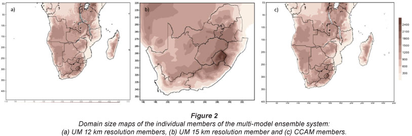
The 12 km no-DA UM forecast covers the subcontinent of southern Africa as well as large areas of the surrounding oceans (Fig. 2a). This configuration runs once a day with 38 levels in the vertical, and produces forecasts 48 h ahead from the initialised field at 00:00 UTC (Tennant, 2007). The forecast output fields are written every hour. This run uses the 18:00 UTC forecast from the UM Global Model to provide initial conditions to the 12 km run at 00:00 UTC, as well as lateral boundary condition fields.
12 km DA
This configuration field has the same domain (Fig. 2a) and resolution as the 12 km no-DA run, but incorporates continuous 3-dimensional variational (3DVAR) DA. DA is a statistical method of combining the latest observational data and the first-guess field from the previous short-range forecast for the same period (Kalnay, 2003). The assimilation process is repeated every 6 h, forecasting 6 h ahead, i.e. 4 times a day, but at the 00:00 UTC assimilation update the model continues to forecast 48 h ahead.
15 km no-DA
The 15 km horizontal resolution run has a much smaller domain (Fig. 2b), than the 12 km resolution runs. It is set up to cover only the South African domain, from 22°S to 35°S and 15°E to 34°E, making it computationally less expensive. This configuration uses no data assimilation, but also uses the 18:00 UTC forecast from the UM Global Model to provide 00:00 UTC initial conditions.
CCAM
The conformal-Cubic Atmospheric Model (CCAM) was developed by the Commonwealth Scientific and Industrial Research Organisation (CSIRO) in Australia (McGregor, 19962005a, 2005b; McGregor and Dix, 2001, 2008). CCAM is a variable-resolution global model, that may be applied either in quasi-uniform mode to function as a global circulation model, or, alternatively, in stretched-grid mode to provide high-resolution forecasts over an area of interest. The model solves the hydrostatic primitive equations using a semi-implicit semi-Lagrangian method (McGregor, 2005). Engelbrecht et al. (2009) and Engelbrecht et al. (2012) have illustrated that CCAM is capable of satisfactorily simulating many attributes of the present-day climatological conditions over southern and tropical Africa. The model has also been shown to produce skilful short-range and seasonal forecasts over the southern African region (Potgieter, 2006; Ghile and Schulze, 2010; Landman et al.,, 2009; Landman et al., 2010, Engelbrecht et al.,, 2011). CCAM became operational at the Council for Scientific and Industrial Research (CSIR) in 2010, so that hindcast data were created in order to perform verification studies for the three summer half-years relevant to this study. In operational mode, the CCAM is initialised at 00:00 UTC, using initial condition fields obtained from the Global Forecast System (GFS). Two different 7-day forecasts are produced daily using the 00:00 UTC initial state. A forecast that has a resolution of about 60 km over southern and tropical Africa is performed first (Fig. 2c). In order to obtain this forecast the model is applied in stretched-grid mode over southern and tropical Africa, with the resolution decreasing to about 400 km in the far-field. A high-resolution forecast is subsequently performed using a more strongly-stretched grid that provides resolution of 15 km over southern Africa, with this run nudged within the 60 km forecast. Hindcasts for the three half-years under consideration were performed using a set-up that mirrors the operational forecasting system. For both the 60 km and 15 km hindcasts, model output is available at 6-hourly time-steps over a domain that covers southern and tropical Africa. All the hindcasts were performed on the Sun Hybrid System of the Centre for High Performance Computing (CHPC) in South Africa.

Rainfall data
South Africa is primarily a summer rainfall region, with only the southwestern Cape being a winter rainfall region (Tyson, 1986). For the three summer seasons under consideration, 24-h rainfall totals were calculated from rain gauge observations originating from automatic and manual weather stations of SAWS and the Agricultural Research Council (ARC). Figure 2 indicates the distribution of the combined observation network of SAWS and the ARC over South Africa, as used in this study. The rainfall totals were accumulated over the 24-h periods from 06:00 UTC on a given day, to 06:00 UTC the next day, in correspondence with the time at which observations are made at manual weather stations managed by SAWS. As all of the NWP forecasts utilised in this study were initialised at 00:00 UTC, the 6 to 30 forecasts corresponding to the rain gauge accumulations were used as a basis for comparison.
In order for the numerical precipitation forecasts to be directly compared to the observed rainfall, the rainfall totals recorded at the weather station locations are processed into a latitude-longitude gridded field. Due to the sparse distribution of stations, it is not meaningful to construct a country-wide grid at a resolution finer than about 0.25°. The rainfall value per grid box at this resolution is calculated, using a box-average technique (Peel and Wilson, 2008), which simply averages all of the rainfall values within the grid box. This procedure has been shown to successfully represent station data on the same grid as that of the numerical weather prediction output (Peel and Wilson, 2008). The number of rainfall stations used in the calculation of the average grid-box value varies across the country with the availability of rainfall stations in the geographical area demarcated by the grid box. In cases where no stations are present within a specific grid box, the grid box is excluded from the subsequent verification calculations. It can be expected that the results of the verification will be sensitive to the number of stations per grid box. For this study, the minimum number of stations required to be present within a grid box was chosen to be 1. With a minimum number of at least 2 stations per grid box, the grid would have fewer samples, particularly in sparsely-covered regions (i.e. Northern Cape), and the results would be skewed toward more populous regions of South Africa (i.e. Gauteng and Western Cape). Even with a grid box represented by only one station, which in turn has the characteristics of a point measurement, making comparison with a model grid box average more problematic, the greater number of valid observational grid boxes was chosen to be the better option for the purpose of this study.
Methodology
Construction of the multi-model ensemble prediction system
An ensemble of forecasts, to some extent, describes the uncertainties pertained in single-model forecasts (Zongjian, 2008; Kalnay, 2003). The multi-model ensemble system (MMENS) presented here is formulated with the purpose of predicting the probability of precipitation exceeding pre-determined thresholds, over a 24-h period, from 06:00 UTC to 06:00 UTC. Although each of the individual members of the multi-model ensemble described in the following sections covers a bigger domain than South Africa (22° to 35°S and 16°E to 33°E), the spatial extent of the SAWS and ARC observational network limits the verification analysis to South Africa. The model output was re-gridded to the same (coarser than the model resolution) horizontal resolution of 0.25° over the South African domain as applicable to the observational data.
Different 24-h rainfall total thresholds are considered in order to formulate dichotomous forecasts for each threshold value: That is, for a given threshold a value of zero is assigned to the forecast if the threshold is not exceeded and a value of 1 if the threshold is exceeded. In this paper the threshold values of daily rainfall totals considered are 1 mm and 10 mm, with the latter representing significant rainfall events. Ebert (2001) noted that a 1 mm/day threshold is useful in the construction of gridded rainfall fields, in order to eliminate dew and insignificant rain. The forecast accuracy and skill in predicting rainfall occurring at or above each of the various thresholds are subsequently investigated.
The MMENS is constructed from the previously mentioned forecasts from the UM and CCAM. The skill of the single-model ensemble forecasts is compared to the MMENS forecasts and the influences of each of the single-model ensemble systems on the MMENS forecast accuracy and skill are described. Only days for which all of the ensemble members are available were used in the analysis.
The individual members of the single-models contribute with equal weights to the respective single-model ensemble systems. The UM ensemble (UMENS) is created by adding the dichotomous forecasts at the grid points for each of the three individual members, and then dividing by N (the number of model configurations - three in this case). Symbolically:

The MMENS is then created by applying equal weights to the two single-model ensemble systems described above.

That is, the output from the UMENS is added to that of the CCAMENS and the total is then averaged, so that both models contribute equally to the MMENS.

Verification metrics
The score for the two thresholds is calculated over the total 18 months of the three summer seasons. For a more detailed description of the results for individual months see Landman (2012).
The forecast bias is calculated in order to determine whether the ensemble systems have a wet (positive) or a dry (negative) bias. The forecast bias (Bias =  explores whether a variable under consideration is systematically over-forecast or under-forecast, and is a measure of forecast accuracy. The perfect forecast would have a bias of 0. Here N represents the total number of forecasts issued for the period considered.
A contingency table (Table 1) approach is used for determining the performance of the dichotomous forecasts by calculating the Frequency Bias Index (FBI; FBI =  Probability of Detection
  FalseAlarm Rate (
 ) and the Critical Success Index (CSI;
  ). Each of these verification scores are calculated for different thresholds. For each forecast or observation for which the threshold is exceeded, the corresponding contingency table value becomes 'yes (or 1)' and 'no (or 0)' if the threshold is not exceeded. The forecast is then analysed using the contingency table which shows the frequency of 'yes' and 'no' forecasts, relative to the observed occurrences (Joliffe and Stephenson, 2003; Wilks, 2006; Fawcett, 2008 - see Table 1). The series of verification statistics obtained in this way, for various threshold values, gives an indication of the forecast's ability to correctly predict the occurrence as well as the amount of rainfall (Ebert, 2001). This process is applied separately to the different ensembles that were formulated. Usually, the contingency tables are set up to explore the average forecast performance over a model domain. This has the disadvantage that the verification scores represent an area average (Ebert, 2001) and cannot distinguish between different geographical locations of the domain or different weather regimes. For this reason, a contingency table is set up for each grid box in the domain, and the scores calculated to present forecast performance at each grid box. In this manner the spatial patterns of the forecast performance can be evaluated. In this paper, only the area-average values will be presented, with the spatial details provided by Landman (2012).

For probability forecasts of dichotomous events the verification metrics consisted of the Brier skill score (BSS; Stanski et al., 1990), the reliability diagram (Jollife and Stephenson, 2003; Wilks, 2006) as well as the relative operating characteristic (ROC; Jollife and Stephenson, 2003; Wilks, 2006). These metrics give almost a complete diagnostic evaluation of forecast performance (Peel and Wilson, 2008).
The BSS (Stanski et al., 1990) is derived from the Brier score (BS; Wilks, 2006, Fawcett, 2008). The BSS answers the question related to the relative skill the probability forecast (predicting whether the event occurred or not) has over that of the persistence (reference) forecast (Mason, 2004). The BS consists of the mean squared error in the probability forecast fi
Here /i assumes a value of 1 if the event was forecast and zero if the event was forecast not to occur. Similarly, a value of 1 is assigned to oi if the event did occur and zero if the event did not occur. The three independent terms of the Brier score are also calculated and are indicated in (2).
Here α is the number of times the events was observed, o, for each of the forecasts made for each probability, Ni, oi is the mean of all of the observations and yi is the mean of all of the forecasts (Wilks, 2006).
The reliability term needs to be as small as possible, which will indicate a well-calibrated forecast because it summarises the conditional bias of the forecast. The resolution term needs to be as large as possible, which will indicate that the forecast resolves the event strongly because it summarises the ability of the forecasts to discern between events. The uncertainty term is only dependent on the climatological frequency of an event occurring and therefore is not influenced by the forecast.
In this paper the BSS is obtained by (3) since it has the advantage of being independent of the manner in which the forecasts are binned, where BSref is the Brier score with persistence as the reference forecast.
The relative operating characteristics determine the discrimination of the forecast between events and non-events. The area under the ROC curve is calculated here with the trapezoid method; this value depends on the degree of separation of distribution of forecast probabilities, conditional on the occurrence of the event from the distribution, conditional on non-events. (Wilks, 2006; Clark et al., 2008; Peel and Wilson, 2008).
The reliability diagram represents the relationship between the observed frequency and the forecast probability of an event (Joliffe and Stephenson, 2003; Wilks, 2006). The reliability diagram is a good companion to the ROC curve, where the reliability diagram is conditioned on the forecast. The reliability diagram shows what the observed frequency is, given the forecast probability for that event to occur.
Together with the reliability diagram, a sharpness or frequency diagram is constructed where the forecast probability bins are plotted against the frequency of the event forecast within each probability bin (over the verification period and at all the grid points). The sharpness diagram is an indication of the confidence of the forecast system under investigation.
Results
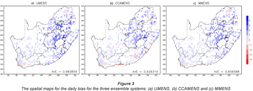
The average bias in predicted 24-h rainfall totals calculated over the three summer seasons for each of the ensemble systems is shown in Fig. 3 (a) to (c). The map of the bias provides insight into the location of areas with relatively high and low, as well as positive (blue shades) and negative (red shades), biases. Considering the three maps, it is noticeable that all three ensemble systems generally have positive biases over the entire domain, indicating too much rain being forecasted. The spatial average bias was calculated for each of the ensemble systems and the value is given on the maps in Figs. 3 (a) to (c). It is seen in Fig. 3 (c) that the CCAMENS has the lowest average bias (0.63 mm/day) of all three systems, whereas the UMENS has the highest daily average bias of ~0.98 mm/day.
Considering the contingency table related scores, the UMENS generally outscores the MMENS with the lower threshold value of 1 mm/day, whereas the MMENS outscores both the single model ensemble systems with the 10 mm/day threshold values. The exception to this is the POD values, where the UMENS has a slightly higher detection rate for the 10 mm/day events than the MMENS (Table 2).

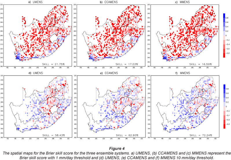
In Fig. 4, the BSS is presented spatially with a score value at each of the grid boxes. Figures 4 (a) - (c) represent the BSS for each of the three ensemble systems for the 1 mm/ day threshold and Figs. 4 (d) - (f) the BSS for the 10 mm/day threshold. On each of the maps, the percentage of grid points with positive BSS values is provided. This number gives an indication of the percentage of grid points over the domain that has skill over that of the persistence (reference) forecast. Therefore, the greater this number, the greater the skill of the forecast is for the 18-month period.
Similar to the scores calculated with the contingency table, the MMENS is outscored by both UMENS and CCAMENS in terms of the percentage positive BSS grid boxes for 1 mm/ day threshold, but it is more skilful than the single-model systems for the 10 mm/day threshold. None of the three systems have any skill over the interior and west-coast of the country in predicting rainfall greater than 1 mm/day but have some skill over persistence for the remaining coastal regions. The MMENS only has 16.6% skilful grid boxes compared to 21.6% for the UMENS at the 1 mm/day threshold, but for the important 10 mm/day threshold the MMENS outscores the two single-model systems, having skill over 72.2% of the total number of grid boxes. The results, as depicted in Fig. 4, have a significant bearing on operational weather forecasting, since they show that there is a better chance of success in forecasting rainfall exceeding the 10 mm/day thresholds as opposed to the low threshold of 1 mm/day. Weather forecasters and other users of NWP rainfall forecasts should therefore take care with the interpretation and use of low threshold value forecasts.
The ROC curves for all three ensemble systems are presented in Fig. 5. In contrast to the low skill determined by the BSS for the 1 mm/day threshold events, the MMENS shows the best discrimination for these events, indicating the multi-model ensemble's improved ability to distinguish between rainfall and non-rainfall events (ROC areas > 0.6). Furthermore, the scores obtained by the MMENS for the 1 mm/day and 10 mm/ day thresholds are comparable, indicating that the MMENS can skilfully distinguish between events and non-events for both thresholds studied.
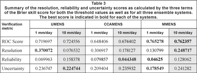
Considering the ROC values in Table 3, it can be argued that the single-model ensemble systems also display good discrimination abilities for both thresholds and that both single-model systems are skilful for these thresholds during the summer season. It is interesting to note that, although the CCAMENS scores systematically lower than the UMENS, the MMENS forecasts are more skilful than any of the constituting single-model ensembles. This result may be due to the CCAMENS having only 3 possible outcomes for each probabilistic forecast at a given location (0, 0.5 or 1), whilst there are 4 possible outcomes for the UMENS and 12 for the MMENS. It is a significant result, which indicates the value of a multi-model ensemble system over single-model systems.
The ROC analysis has shown that the MMENS system is the most suitable to discriminate between rainfall events exceeding predetermined thresholds and events that do not reach these thresholds. Hence, reliability diagrams are only presented for this system (Fig. 6). The diagram shows that the MMENS system exhibits over-confidence for both thresholds. Considering the 1 mm/day threshold (blue line) the system is under-forecasting the events with low probabilities and over-forecasting for higher probabilities (< 70%). The 10 mm/day threshold (green line) has slightly better reliability but is over-forecasting the events with probabilities > 30%. The sharpness diagrams in Fig. 6 show that for both thresholds the MMENS has high confidence. In all of the threshold events, the highest number of forecasts is made in the lower probability bins, with some increase with the 10 mm/day threshold events in the higher probabilities.

In order to accurately determine the difference between the three systems, the reliability, resolution and uncertainty are calculated for both threshold values and represented in Table 3. For the events exceeding the 10 mm/day threshold, the MMENS has a better resolution, but for those events exceeding 1 mm/day, the UMENS has better resolution. For reliability, the MMENS outscores at the lower threshold, but the CCAMENS is the most reliable of the three systems with 10 mm/day events. The same holds true for the uncertainty of the systems, except that the uncertainty is the lowest with the UMENS at 10 mm/ day threshold.
In terms of the skill for each of the ensemble systems, the three systems are skilful in predicting rainfall for the South African domain. However, all three of the systems are less skilful in predicting low threshold events (1 mm/day) compared to higher threshold (10 mm/day) events. The multi-model's ability to distinguish between events and non-events is greater than that of the two single-model ensemble systems. The multi-model ensemble system can possibly be improved by removing the model errors through increased ensemble members as well as through the use of a weighted combination method that considers the relative skill of the individual contributing ensemble members.
Discussion and conclusions
Weather forecasters at operational centres such as SAWS are often faced with the challenge of making reliable site-specific probabilistic rainfall forecasts for the next day or two. The forecaster is presented with different forecasts, either from different configurations of the same weather forecast model, or from different models or a combination of both. The forecaster has to combine the various forecast outputs into a probability statement, which is done in a highly subjectively way and is often based on a forecaster's own perceptions or preference for a particular model. A method combining forecasts through a simple un-weighted approach into a single objective probability forecast is presented here. These forecasts were verified over three 6-month summer seasons.
The results show that combined forecasts from different forecast systems generally outscore forecasts from the individual models. Care should however be taken when using this multi-model system in predicting low threshold values (i.e. 1 mm/day). In fact, the systematic overestimation of rainfall by all three ensemble systems over the interior of South Africa, the absence of skill in predicting the occurrence of rainfall above the 1 mm threshold event, and relatively poor performance of all systems in predicting events above the 10 mm threshold over the central interior of South Africa, warrant research into the improvement of convective rainfall parameterisations, and, perhaps the application of non-hydrostatic models at very high resolution, over South Africa (e.g. Engelbrecht et al., 2007). The paper has also demonstrated the attributes of combining forecasts produced by different institutions running different forecast models, and therefore suggests that additional models' outputs may be considered for inclusion in a multi-model system for further improved operational weather forecasting in South Africa. Additional forecast outputs to consider includes forecasts from the Weather and Research Forecast model (to be used is operational model at SAWS and also run at the University 3f Pretoria), the NCEP ensemble, and possibly forecasts from the European Centre for Medium-Range Weather Forecasts. However, for the system in this study to be optimised fully, it will be necessary for the model errors identified to be corrected within each of the ensemble members, before constructing an improved multi-model system.
Apart from improving on model physics and numerical schemes, future NWP research in South Africa should address the best way to weight forecasts form different models, down-scaling or recalibrating forecasts (since it was shown here that the different models have different systematic errors), and the use of larger forecast ensembles. In addition, the use of even tiigher resolution forecasts beyond the hydrostatic limit should be considered, as convective rainfall is such a dominant feature 3f South Africa's climate, and the value of more advanced data assimilation techniques quantified.
Acknowledgements
The South African Weather Service provided funding this research, and both SAWS and ARC provided the rainfall data used as basis for verification. The Water Research Commission, through Project K5/1646, funded the creation of the CCAM riindcast data used in this study. We would like to thank the CHPC for their excellent support whilst performing the large set of CCAM hindcasts.
References
BAKHSHAII A and STULL R (2009) Deterministic ensemble forecasting using gene-expression programming. Weather Forecast. 24 1431-1451. [ Links ]
BOWLER NE, ARRIBAS A, MYLNE KR, ROBERTSON KB and BEARE SE (2008) The MOGREPS short-range ensemble prediction system. Quart. J. R. Meteorol. Soc. 134 703-722. [ Links ]
CLARK AJ, GALLUS WA and CHEN T (2008) Contributions of mixed physics versus perturbed initial/lateral boundary conditions to ensemble-based precipitation forecast skill. Mon. Weather Rev. 136 2140-2156. [ Links ]
DAVIES T, CULLEN MJP, MALCOLM AJ, MAWSOM MH, STANIFORTH A, WHITE AA and WOOD N (2005) A new dynamical core for the MetOffice's global and regional modelling of the atmosphere. Quart. J. R. Meteorol. Soc. 131 1759-1782. [ Links ]
EBERT EE (2001) Ability of a poor man's ensemble to predict the probability and distribution of precipitation. Mon. Weather Rev. 129 2461-2480 [ Links ]
ENGELBRECHT FA, McGREGOR JL and ENGELBRECHT CJ (2009). Dynamics of the conformal-cubic atmospheric model projected climate-change signal over southern Africa. Int. J. Climatol. 29 1013-1033. DOI: 10/1002/joc.1742. [ Links ]
ENGELBRECHT CJ, ENGELBRECHT FA and DYSON LL (2012) High-resolution model-projected changes in mid-tropospheric closed-lows and extreme rainfall events over southern Africa. Int. J. Climatol. DOI: 10.1002/joc.3240. [ Links ]
ENGELBRECHT FA, LANDMAN WA, ENGELBRECHT CJ, LANDMAN S, BOPAPE MM, ROUX B, McGREGOR JL and THATCHER M (2011) Multi-scale climate modelling over Southern Africa using a variable-resolution global model. Water SA 37 (5) 647-658. [ Links ]
ECKEL FA and MASS CF (2005) Aspects of effective mesoscale, short-range ensemble forecasting. Weather Forecast. 20 328-350. [ Links ]
FAWCETT R (2008) Verification techniques and simple theoretical forecast models. Weather Forecast. 23 1049-1068. [ Links ]
FRIEDERICHS P and HENSE A (2008) A probabilistic forecast approach for daily precipitation totals. Weather Forecast. 23 659-673. [ Links ]
GHILE YB and SCHULZE RE (2009) Evaluation of three numerical weather prediction models for short and medium range agrihydrol-ogy applications. WaterResour. Manage. 24 1005-1028. [ Links ]
GRIMIT EP and MASS CF (2002) Initial result of a mesoscale short-range ensemble forecasting system over the Pacific Northwest. Weather Forecast. 17 192-205. [ Links ]
HAMILL TM and COLUCCI SJ (1997) Verification of Eta-RSM short-range ensemble forecasts. Mon. Weather Rev. 125 1312-1327. [ Links ]
JOLIFFE IT and STEPHENSON DB (2003) Forecast verification: A practitioner's guide in atmospheric sciences. John Wiley & Sons Ltd, England. 1630 pp. [ Links ]
KALNAY E (2003) Atmospheric Modeling, Data Assimilation and predictability. Cambridge University Press, Cambridge. [ Links ]
LANDMAN S, ENGELBRECHT FA, ENGELBRECHT CJ, LANDMAN WA and DYSON LL (2010) A multi-model ensemble system for short-range weather prediction in South Africa. Proc. 26th Annual Conference of the South African Society for Atmospheric Sciences, September 2010, Gariep Dam. ISBN 978-0-620-47333-0. [ Links ]
LANDMAN S (2012) A multi-model ensemble system for short-range weather prediction in South Africa. M.Sc. thesis, University of Pretoria, Pretoria. 137 pp. [ Links ]
LEWIS JM (2005) Roots of ensemble forecasting. Mon. Weather Rev. 133 1865-1885. [ Links ]
LORENZ EN (1963) Deterministic nonperiodic flow. J. Atmos. Sci. 20 130-141. [ Links ]
MASON SJ (2004) On using "climatology" as a reference strategy in the brier and ranked probability skill scores. Mon. Weather Rev. 132 (7) 1891-1895. [ Links ]
McGREGOR JL (2003) A new convection scheme using simple closure. In: Current Issues in the Parameterizations of Convection. BMRC Research Report 93. 36-36. [ Links ]
McGREGOR JL (2005) C-CAM: Geometric aspects and dynamical formulation. CSIRO Atmospheric Research Tech. Paper No. 70. CSIRO, Australia. 43 pp. [ Links ]
PEEL S and WILSON LJ (2008) A diagnostic verification of the precipitation forecasts produced by the Canadian ensemble prediction system. Weather Forecast. 23 569-616. [ Links ]
POTGIETER CJ (2006) Short-range weather forecasting over southern Africa with the conformal-cubic atmospheric model. M.Sc. thesis, University of Pretoria, Pretoria. 172 pp. [ Links ]
ROY BHOWMIK SK and DURAI VR (2010) Application of mul- timodel ensemble techniques for real time district level rainfall forecasts in short range time scale over Indian region. Meteorol. Atmos. Phys. 106 19-35. [ Links ]
STAËL VON HOLSTEIN CS (1971) An Experiment in probabilistic weather forecasting. J. Appl. Meteorol. 10 635-645. [ Links ]
STANSKI HR, WILSON LJ and BURROWS WR (1990) Survey of common verification methods in meteorology. WMO World Weather Watch Tech. Rep. 8 WMO TD 358. 114 pp. [ Links ]
STENSRUD DJ and YUSSOUF N (2005) Bias-corrected short-range ensemble forecasts of near surface variables. Meteorol. Appl. 12 217-230. [ Links ]
STENSRUD DJ, BROOKS HE, DU J, TRACTON S and ROGERS E (1999) Using ensembles for short-range forecasting. Mon. Weather Rev. 127 433-446. [ Links ]
TENNANT WJ, TOTH Z and RAE KJ (2007) Application of the NCEP ensemble prediction system to medium-range forecasting in South Africa: New products, benefits, and challenges. Weather Forecast. 22 18-35. [ Links ]
THEIS SE, HENSE A and DAMRATH U (2005) Probabilistic precipitation forecasts from a deterministic model: A pragmatic approach. Meteorol. Appl. 12 257-268. [ Links ]
TOTH Z, XHU Y and MARCHOK T (2001) The use of ensembles to identify forecasts with small and large uncertainties. Weather Forecast. 16 463-477. [ Links ]
TYSON PD (1986) Climate Change and Variability over Southern Africa. Oxford University Press, Cape Town. [ Links ]
WANDISHIN MS, MULLEN SL, STENSRUD DJ and BROOKS HE (2001) Evaluation of a short-range ensemble system. Mon. Weather Rev. 129 729-747. [ Links ]
WILKS D (2006) Statistical Methods in the Atmospheric Sciences (2nd edn.). Elsevier Academic Press, California. [ Links ]
ZONGJIAN KE, DONG W and ZHANG P (2008) Multimodel ensemble forecasts for precipitation in China in 1998. Adv. Atmos. Sci. 25 72-82. [ Links ]
Received 3 February 2012; accepted in revised form 1 October 2012.
* To whom all correspondence should be addressed. +27 12 367 6054; fax: +27 12 367 6189; e-mail: stephanie.landman@weathersa.co.za

