


Services on Demand
Article
 English (pdf)
 Article in xml format
 Article references
Indicators

Related links
-
 Cited by Google
 -
 Similars in Google
Share

 Permalink
Water SA
On-line version ISSN 1816-7950
Print version ISSN 0378-4738
Water SA vol.38 n.2 Pretoria Jan. 2012
ARTICLES
Sensitivity study of reduced models of the activated sludge process, for the purposes of parameter estimation and process optimisation: Benchmark process with ASM1 and UCT reduced biological models
S du Plessis; R Tzoneva*
Department of Electrical Engineering, Cape Peninsula University of Technology, Cape Town, South Africa
ABSTRACT
The problem of derivation and calculation of sensitivity functions for all parameters of the mass balance reduced model of the COST benchmark activated sludge plant is formulated and solved. The sensitivity functions, equations and augmented sensitivity state space models are derived for the cases of ASM1 and UCT reduced biological models. Matlab software for sensitivity function calculation and sensitivity model simulation is developed. The results are described and discussed. The behaviour of the sensitivity functions is used to determine which parameters of the reduced model need to be estimated in order to fit the reduced model behaviour to the real data for the process behaviour.
Keywords: wastewater treatment, activated sludge process, reduced model, model parameters, sensitivity function, Matlab simulation
Introduction
The problem of effective and optimal control of wastewater treatment plants has become very important in recent years due to increased populations and requirements for the quality of the effluent. The activated sludge process (ASP) is a waste-water treatment process characterised by complex nonlinear dynamics, a large number of variables, and a lack of sensors for real-time measurement of many of these variables. The above process characteristics require real-time control design and implementation strategies to be developed in order to achieve process operation which is compliant with the international standards for effluent quality. Modern optimal control design and implementation for the activated sludge process demands extensive insight into the plant's operation, clear objectives, and knowledge about process dynamics described by an appropriate mathematical model. Modelling is the most critical phase in the solution of any control problem because nearly all control techniques require knowledge of the dynamics of the system before control design can be attempted. This means that the primary task of any modern control design is to construct and identify a model for the system which is to be controlled.
Mathematical models of the wastewater treatment processes were developed using the first principles of conservation of mass and energy (Copp, 2002), on the basis of developed biological models, such as the first ones described by Dold et al. (1980), Henze et al. (1987) and Wentzel et al. (1992). The obtained mass-balance models describe the process-technology structure and biological reactions taking part in this structure.
Examples of such models are the COST benchmark model (Copp, 2002) and the University of Cape Town (UCT) model (Ekama and Marais, 1979; Ekama et al., 1984). The most used biological models are the IAWQ1 (Henze et al., 1987) - the model of the International Association for Water Quality called Activated Sludge Model 1 (ASM1), and the UCT model - the model developed at the UCT Department of Civil Engineering (Dold et al., 1980).
The full ASM1 and especially the UCT model present major problems in terms of their direct use for real-time simulation and control design purposes, because of their complexity, limitations and drawbacks, as follows:
- Large number of model variables
- Complex dependencies and interconnections between the biological variables
- Different time scales for the process dynamics
- The control actions for the process are not included in an explicit way in the model equations
- Many variables are difficult to measure
- Many model kinetic and stoichiometric parameters are difficult to determine and have uncertain values
A way to overcome these difficulties would be to simplify the complex model by developing reduced biological and mass-balance models with a small number of variables, while still maintaining the same characteristics as these of the original full model (Pearson, 2003). Kinetic parameters of this reduced model can be determined by development and application of different methods for parameter estimation (Holmberg and Ranta, 1982; Jeppson, 1996; Halevi et al., 1997; Noykova and Gyllenberg, 2000).
Solution of the problem of parameter estimation is based on the given mathematical model in which the parameters are not known, and on data for the process variables obtained by measurement. Many of the biological nutrient removal models are not identifiable since they have many more parameters than feasible measurements (Pertev et al., 1997; Varma et al., 1999). In this case the problem can be solved if the influence of the parameters on model behaviour is studied and the non-influential parameters are considered to have zero or constant known (nominal) values. The influential parameters can then be estimated on the basis of data from the measurements (Varma et al., 1999). The goal of the paper is to develop a mathematical and computational tool for determining which parameters can be accepted as known and which need to be estimated on the basis of the reduced model of the COST benchmark process (Du Plessis, 2009).
A sensitivity study of the model variables towards the model parameters provides a tool to identify the influential parameters. The sensitivity study of the dynamic model set of equations examines the changes in the model variables in response to changes in the model parameters (Smets et al., 2002; Mussafiet et al., 2002; De Pauw and Vanrolleghem, 2003). Parameters resulting in large values for the sensitivity function have to be estimated (Sato and Ohmori, 2002; Louries et al., 2008). If some parameters with small values for the sensitivity function could be found, the problem of parameter estimation could be simplified by considering these parameters as known (Holmberg and Ranta, 1982; Noykova and Gillenberg, 2000).
There are different mathematical methods for parametric sensitivity analysis, such as finite difference, direct, the Green's function, the polynomial approximation, and so on. Most previous studies have used the finite difference method (Smets et al., 2002; Plazl et al., 1999; Mussafiet at al., 2002; Varma et al., 1999; Pertev et al., 1997). This method is calculation-intensive and gives a local estimation of the sensitivity function for a given parameter. The global sensitivity method simultaneously calculates the sensitivity functions for a large number of parameters and for a large variety of parameters. This method allows better analysis of the parameter's influence as it provides full information about each sensitivity function. The direct method is applied for the mass balance model of the COST benchmark plant (Copp, 2002), based on ASM1 and UCT reduced biological models, developed in Du Plessis (2009). The mass balance models are used for derivation of the sensitivity functions of the model variables towards all kinetic and stoi-chiometric model parameters. As a result, a dynamic sensitivity state-space model is developed. The reduced process model is augmented with the sensitivity model in order to build a model giving possibilities for global sensitivity analysis of all model variables to all model parameters. Matlab software for sensitivity function calculation and global (augmented) sensitivity model simulation is developed. The results are described and discussed.
First, a definition of the sensitivity functions is given. Reduced ASM1 and UCT biological and benchmark mass balance models are then described. The augmented sensitivity state-space model of the benchmark mass balance reduced model, based on the ASM1 biological model and based on the UCT biological model, is derived further. Description of Matlab software and results from simulation of the above models are given followed by discussion of the results. Finally, a summary of the results is given and their importance and applicability discussed.
Sensitivity functions, vectors and models
The behaviour of physical systems is determined by the values of their parameters. Investigation of the system response to changes in the values of the parameters enables determination of parametric sensitivity. Such analysis is important for all spheres of science and engineering, especially for design of the systems and their control (Frank, 1978; Varma et al.,1999; Fesso, 2007). The sensitivity functionXθ(t) of the nonlinear system:

where:
XЄRl is the state space vector,
uЄRm is the control vector,
gЄRl is the nonlinear vector function of the process states, controls and parameters, and
θЄRp is the vector of the parameters, is defined as (Sato & Ohmori, 2002):

In other words, the sensitivity function (Xθij) is a mathematical description which indicates the influence of a slight change in parameter θj on the behaviour of the state variable Xi and XθЄRl. Differentiating (1) according to the vector θ gives the sensitivity dynamic nonlinear equation:

The solution of the Eq. (3) describes the sensitivity function behaviour, but requires data for the state-space variables of the model given by Eq. (1). This means that a set of Eq. (1) and (3) has to be solved simultaneously. The set of these 2 equations can be represented as an augmented mathematical model (Tzoneva et al., 1996). The augmented sensitivity model is obtained by extension of the model state-space vector by the vector of the sensitivity func-tions, as follows:
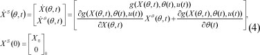
The augmented model is used for global parametric analysis of the reduced COST benchmark mass balance model for the case of the ASM1 and UCT reduced biological models. Equations (1)-(4) are derived for each of these 2 cases.
Reduced biological and mass balance models for cost benchmark plant layout
Reduced biological models
A fundamental requirement for development of reduced models is that they contain a minimum number of state variables and parameters to allow for model identification based on available online measurements and for online calculation of the process optimal control. Different types of reduced models are introduced in the literature (Moore, 1981; Glover, 1984; Safanov and Chiang, 1989; Latham and Anderson, 1985; Al-Saggaf and Franklin, 1988; Wisnewski and Doyle, 1996; Halevi et al., 1997; Beck et al., 1996; Lee at al., 2002; Jeppson, 1996) using different approaches of reduction, such as qualitative analysis, truncation methods, dominant eigenvalues, and optimisation.
The existing biological models of the activated sludge process are characterised by a large number of processes and compounds, as well as a large number of kinetic and stoichiometric parameters. These models, such as ASM1 and UCT, are very complex for use in real-time state and parameter estimation and process optimisation. ASM1 and UCT reduced models, used in conjunction with the benchmark mass balance model, are developed in Du Plessis (2009), applying time-scale analysis of the model variables' dynamics (Dochain, 2003; Lennox et al., 2001; Stecha et al., 2005; Wang and Gawthrop, 2001). This allows decomposition of the complex models' variables into the following time scales:
- Fastest (minutes) - dynamics of physical-chemical variables such as dissolved oxygen, pH, conductivity, redox potential
- Intermediate (hours) - dynamics of utilisation of carbonaceous and nitrogenous substrates and the inflow flow rate and concentrations of waste materials
- Slowest (weeks or months) - dynamics of the heterotrophic and autotrophic microorganisms and slowly biodegradable biomass
The main disturbances to the activated sludge process are the load disturbances determined by the inflow rate and waste concentrations. The control of the ASP would be effective if it could overcome the effect of the inflow disturbances. This means that the model of the process has to have dynamics within the same time scale as that of the disturbances. That is why only dynamics of the carbonaceous and nitrogenous substrate and inflow disturbances are included in the reduced model. It is possible to neglect the equations of the full biological model describing the concentrations of the slowest variables because their dynamics are many times slower and they can thus be considered to be in a steady state. It is also possible to neglect the equation for dissolved oxygen (DO) concentration because its dynamics are approx. 10 times faster than the dynamics of the substrate concentrations, and it can be assumed that the value of the DO is controlled and is equal to that of the required set-point. The dissolved oxygen concentration as a control variable is included in the switching functions of the process rates describing the reduced models. The above principles are used for development of both the ASM1 and UCT reduced models. At the same time the differences between them, due to the different views on the processes of adsorption and hydrolysis, are preserved. The notations of the ASM1 model are used for the process variables of both models. The notations of the model parameters are kept as for the original models.
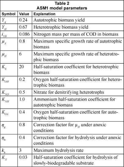
Reduced-order ASM1 biological model
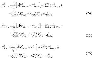
Aerobic growth of heterotrophs XBH for degrading of organic matter, anoxic growth of heterotrophs for the de-nitrification process, aerobic growth of autotrophs XBA for the nitrification process and, lastly, the hydrolysis of entrapped organic nitrogen, are the processes that characterise the dynamic behaviour of the 3 components used in describing the removal of carbon and nitrogen: soluble ammonium nitrogen SNHn. soluble nitrate nitrogen SNOn and soluble readily-biodegradable substrate SSn concentrations. This model is described by the Peterson matrix given in Table 1. It has 4 processes and 3 compounds (vari-ables), where SOn is the concentration of dissolved oxygen and XSn is the slowly-biodegradable substrate concentration. The typical values of the model parameters for the ASM1 model are given in Table 2.
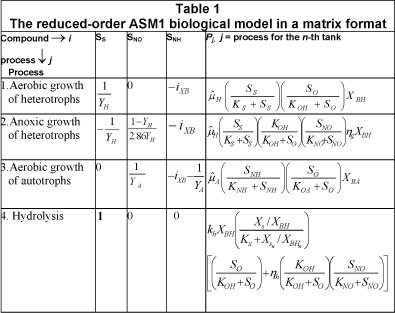
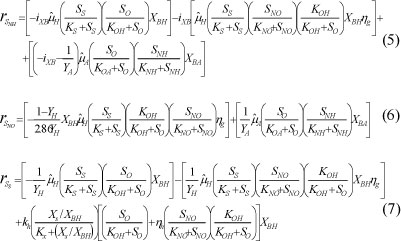
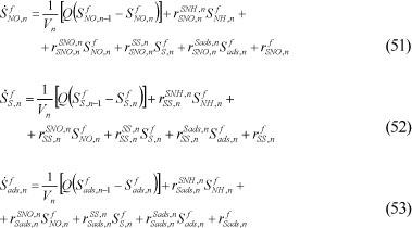
The corresponding differential equations describing the variables’ rates for the n-th tank are:
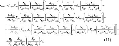
Reduced-order UCT biological model
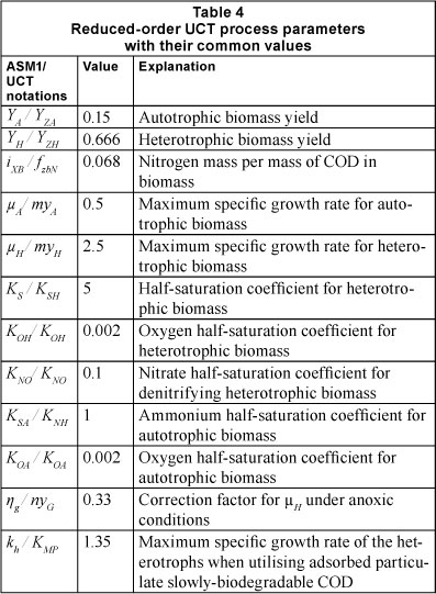
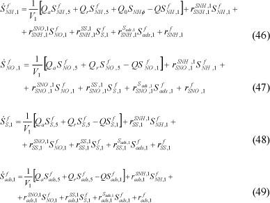
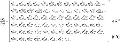
The model is described by the Peterson matrix given in Table 3. It has 10 processes and 4 variables. The considered processes are: aerobic growth of XBH on Ss with SNH, aerobic growth of XBH on SS with SNO, anoxic growth of XBH on SS with SNH, anoxic growth of XBH on SS with SNO, aerobic growth of XBH on Sads with SNH aerobic growth of XBH on Sads with SNO, anoxic growth of XBH on with SNH , anoxic growth of XBH on Sads with SNO, adsorption of XS , aerobic growth of XBA on SNH. The additional variable, representing the main concept of the enzyme reactions in the UCT model is Sads, which describes the concentration of the adsorbed slowly-biodegradable substrate. The model parameters are given in Table 4. The UCT notations for the model parameters are used.
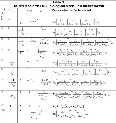
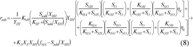
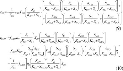
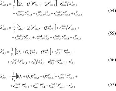
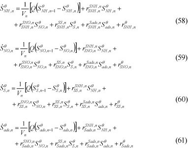
The corresponding equations for the variables' rates are:
Mass-balance reduced model of the benchmark plant
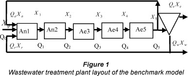
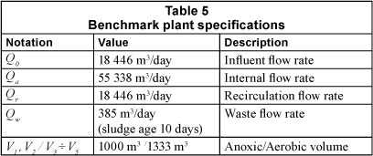
The layout of the COST benchmark structure (Copp, 2002) is given in Fig. 1. The benchmark format has 2 anoxic tanks, 3 aerobic tanks and a secondary settler with 2 recycle flows (from aerobic tank 5 to the input and from the settler to the input), where: Q0 is the input flow rate, Qa is the internal recycle flow rate, Q n=1:5, is the output flow rate of the n-th tank, Qr is the recycle flow rate, Qe is the effluent flow rate, and Qw is the waste flow rate,Xn n=1:5, is the vector of the waste compound concentrations in the influent and the n-th tank. The values of the flow rates and tanks volumes are given in Table 5.
The sensitivity of the reduced model variables towards the model parameters is evaluated by using the theory of sensitivity (Schermann and Garag-Gabin, 2005; Montgomery, 1997; Breyfogle and Breyfogle, 2003).
The mass-balance equations describing the benchmark structure for the reduced ASM1 and UCT biological models in discrete time domain are (Du Plessis, 2009):
For Tank 1: where Q = Qa + Qr + Q0
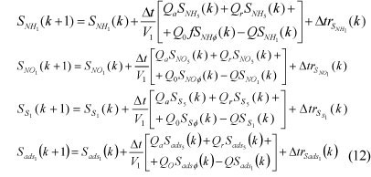
For Tank n=2, 3, 4, and 5:
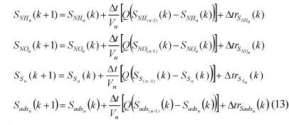
where:
Xn=[SNHn SNOn SSn]T and
Xn=[SNHn SNOn SSn Sadsn]T,
n=1:5, are vectors of the concentrations of the variables considered in the ASM1 and UCT reduced models, and Δt=15 (min) is the sampling period. The model of the settler, considered as an ideal one, is incorporated in the above equations as:

where:
for the soluble compounds, λ=1, and for the particulate compounds, λ=(Q0+Qr)/(Qr+Qw).
The above equations are the same for both the ASM1 and UCT model, as structure, flow and volume. The difference is in the description of the number of compounds and the process rates, due to the different approaches to representing the biological activities of the microorganisms in these 2 models (Wentzel et al., 1992). The variables’ rates r are described correspondingly by Eqs. (5) ÷ (7) for the reduced ASM1 and by Eqs. (8)÷(11) for the reduced UCT model.
Additionally to the parameters of the reduced models, a parameter f is included in the mass balance equations for the 1st tank. This parameter multiplies the concentration of the ammonia nitrogen in order to take account of the biological ammonia not considered in the reduced models, due to neglecting of the variable SND (soluble biodegradable organic nitrogen concentration).
The sensitivity of the reduced model variables towards the model parameters is evaluated by using the theory of sensitivity (Schermann and Garag-Gabin, 2005; Montgomery, 1997; Breyfogle and Breyfogle, 2003).
Augmented sensitivity mass balance model derivation for the case of ASM1 reduced model
Sensitivity functions and equation derivation
The derivations of the sensitivity functions and models are analogous for every process tank. That is why they are calculated for the n-th tank, as follows:
For the parameter f
1) For the 1st tank
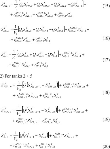
dSNH,n/df=SfNH,n' dSNO,n/df=SfNO,n' dSs,n/df=Sfs,n are the sensitivity functions of the process variables towards the parameter f. The variables' rate derivatives towards the process variables
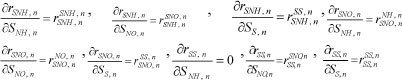
are given in Appendix A.
- For the parameters

1) For the 1st tank
2) For the tanks n = 
where:
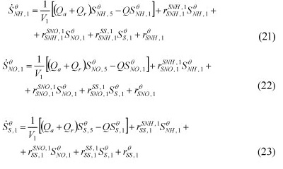
Sθ, NH,n' SθNO,n' SθS,n are the sensitivity functions to the parameter q, the partial derivatives of the variable’s rates according to the variables are determined above and the derivatives of the variables’ rates according to the model parameters are given in Appendix A.
Augmented sensitivity state-space model
The sensitivity state-space model is derived for the whole plant. The vector of the sensitivity state-space consists of all sensitivity functions according to the model parameters, as follows for the n-th tank:
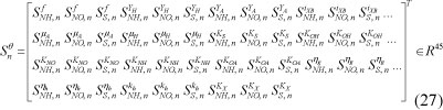
The state process variables’ vector for the n-th tank is:

The combined vector for the process variables and sensitivity functions for the n-th tank is:

This vector is used for the augmented state-space process and sensitivity-function model derivation.
The matrix of the derivatives of the variables’ rates towards the process variables is:

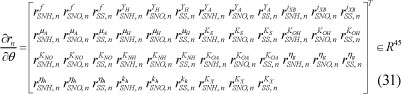
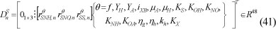
The vector of the derivatives of the process rates to the model parameters, Appendix A, is:
Description of the augmented model in the discrete state-space domain is given for every tank separately because of the large dimensions of the vector of the state-space.
- Augmented sensitivity state-space equation for the 1ª tank in the discrete form incorporates the process variables and sensitivity functions, as follows:
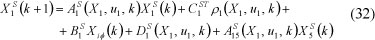
where:
the variables' rates are expressed by the process rates rI(k)=ClSTpl(k), and pl=[p11 p12 p13...p1N[T is a vector of the process rates, ul(k)=S0,1(k) is the dissolved oxygen concentration in the 1ª tank, considered as its control action:
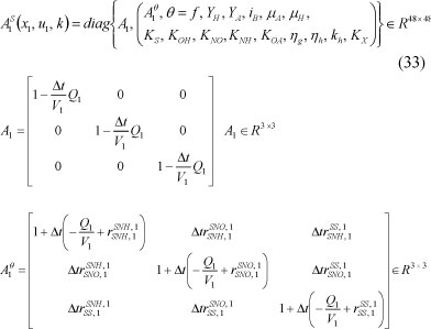
The matrices A1θ are identical for all parameters. The matrix ClSrepresents the parameters in the Peterson matrix and is:
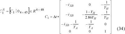
The matrix BlS is:
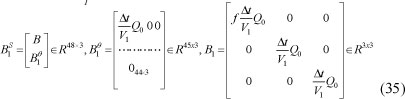
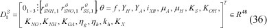
The inflow variables' concentration vector is XiØ=[SNHØ SNOØ SSØ]T. The vector DlS represents the derivatives of the variables' rates towards the model parameters.
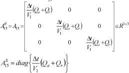
are done by the vector X5S=[X5 S5Ø]ЄR48:
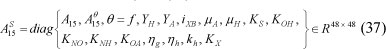
where:
all matrices A15 are identical and:
- Augmented sensitivity model equations for tanks n = 2 ÷ 5
The state-space model inc orporating the pro c e s s variable s and sensitivity functions are derived for the n-th tank, as follows:

where:

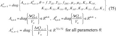
The matrices An,n-1S are:
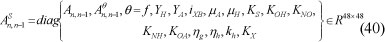
where:
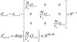
The vector Dsns:
The matrices CnS are equal to C1S.
- Augmented sensitivity state-space model of the whole plant
The model of the variables and sensitivity functions for the whole plant is described on the basis of Eqs. (32) and (38) as follows:

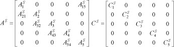
The matrices ASЄR240x240 and CSЄ R20x240 are:
The vector of the process rates is:

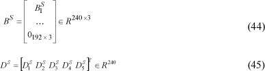
The matrix BS and the vector DS are:
Model (42)-(45) is used to calculate the parametric sensitivity functions of the benchmark structure with the ASM1 reduced model.
Augmented sensitivity mass balance model derivation for the case of the UCT reduced-order model
Sensitivity function and equation derivation
The order of calculation is done in the same way as above.
- For the parameter f
1) For the 1st tank
The sensitivity functions are given by equations:
2) For the other n = 2÷5 tanks
The sensitivity functions are given by the equations:

- For the parameters

the equations are as follows:
1) For the 1st tank
2) For the tanks n = 2 ÷ 5
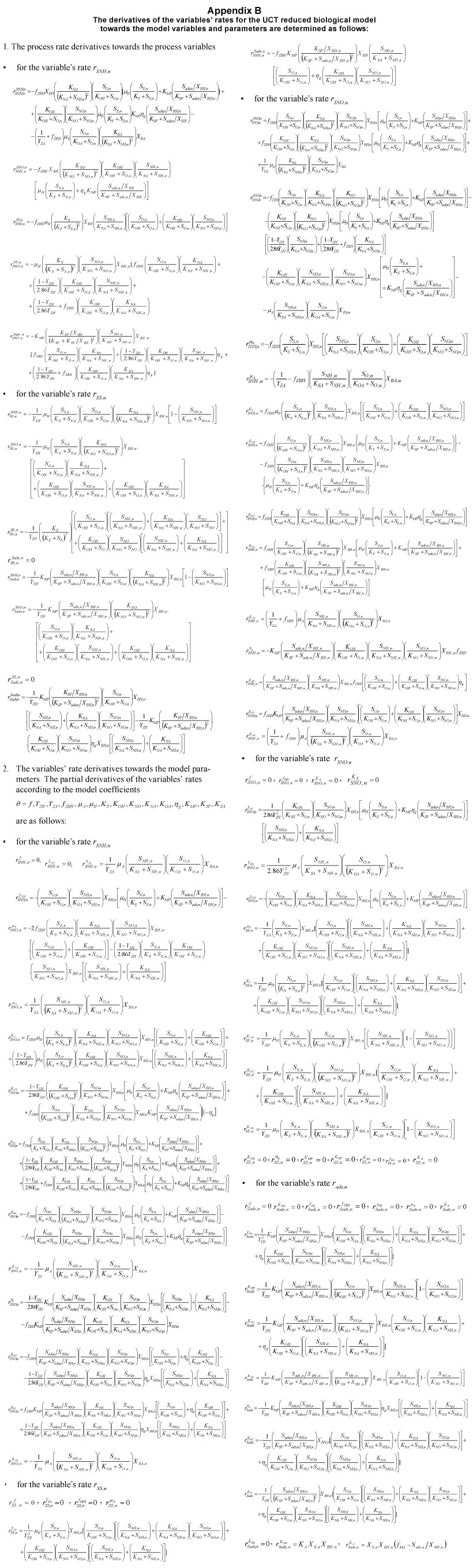
The partial derivatives of the variables’ rates are determined in Appendix B.
Augmented sensitivity state-space model
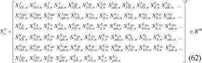
The augmented sensitivity state-space model is formed in the same way as above. It is based on the model of the plant extended with the model of the sensitivity functions. The vector of the sensitivity functions consists of all sensitivity functions according to the model parameters, as follows for the n-th tank:
The process state-space vector for the n-th tank is:

The augmented vector for the process variables and sensitivity functions is:

This vector is used to describe the augmented model of the process variables and sensitivity functions. The matrix of the process variables’ rates derivatives towards the process variables is:

The partial derivatives of the variables' rates are determined in Appendix B.
The augmented process and sensitivity state-space model is described for every tank separately because the large dimension of the vector of state-space and the number of tanks creates the need for a large amount of space for describing the model matrices.
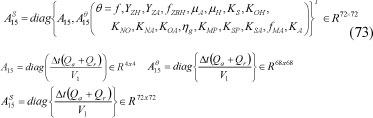
- The state-space model for Tank 1 in discrete form is:
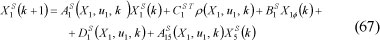
where:p1=[p11 p12 p13 ... p1,10]T is a vector of the process rates
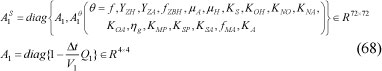
The matrices A1θ èare identical for all model parameters:
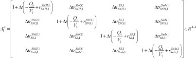
The matrix C1 S=[C1 010x68]∈¸R10x72 represents the parameters from the Peterson matrix:
The inflow vector is:

The vector D1Srepresents the derivatives of the variables' rates towards the model parameters:

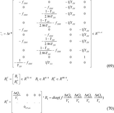
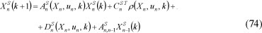
The matrix A15Sdescribes the internal recycle between the end of the 5th tank and the beginning of the 1st one. The vector X5Sis formed in the same way as the vector X1S : X5S=[X5 S5θ]TЄR72 where:
- Derivation of the equations for tanks n = 2 ÷ 5
The return-flow dynamics for all other tanks are identical, thus the models will have the same structure, as follows:
where:
The matrix Anθ has the same structure for all parameters θ and for all tanks n=2:5.
The matrices An,n-1 S are:
The matrices CnS are equal to ClS with the same coefficients.
The vector DnS is:

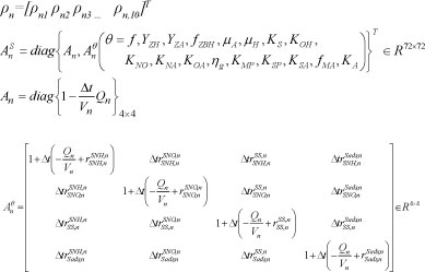
- Augmented sensitivity state-space model of the whole plant Combining all equations for the tanks, the full model is:
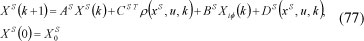
where:
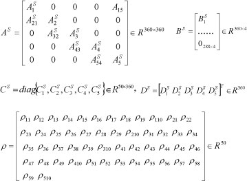
The augmented model (77) is used for calculation of the sensitivity functions of the COST benchmark plant reduced mass-balance model for the case of the UCT reduced biological model. The models (42) and (77) are nonlinear because of the nonlinear rate expressions in the matrices AS and vectors r and DS. The dissolved oxygen concentration is considered as a control input for these models and it appears in the rate expressions forming AS, r, and DS. Matlab programs are developed for parameter sensitivity calculations using equations (42) and (77). A matrix/vector representation of the models allows simplification of the software code and reduction of time for calculations.
Sensitivity analysis
The sensitivity analysis of the wastewater treatment model variables towards the model parameters is done in order to determine which parameters have to be estimated for the corresponding reduced models during the real-time operation and control of the process.
Software for the sensitivity analysis
Software programs are developed in the Matlab environment for the considered 2 cases:
- Calculation of the sensitivity functions of the benchmark process based on ASM1 reduced biological model: programs BASM1S.m, rateASM1.m
- Calculation of the sensitivity functions of the benchmark process based on UCT biological model: programs BUCTS1.m, rateBUCTS.m
- For each of the considered cases the software consists of:
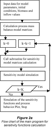
- Main program for input of the nominal process parameters, initial conditions, average values of the biomass concentrations, calculation of the process model matrices and organisation of the calculation algorithm
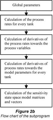
- Sub-programs for calculation of the process rates, sensitivity functions and formation of the sensitivity model state-space and rate matrices and vectors.
The algorithm of the calculation is given in Fig. 2a for the main programme and in Fig. 2b for the sub-programmes.
Results for the ASM1 reduced biological model
Simulation is done for the parameters given in Table 3 and for the inflow average concentration given by the vector Xθ:

The steady-state conditions of the biomass and the slowly-biodegradable substrate are given by the vectors:
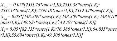
The vector of the dissolved oxygen concentration is:

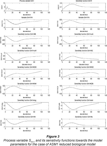
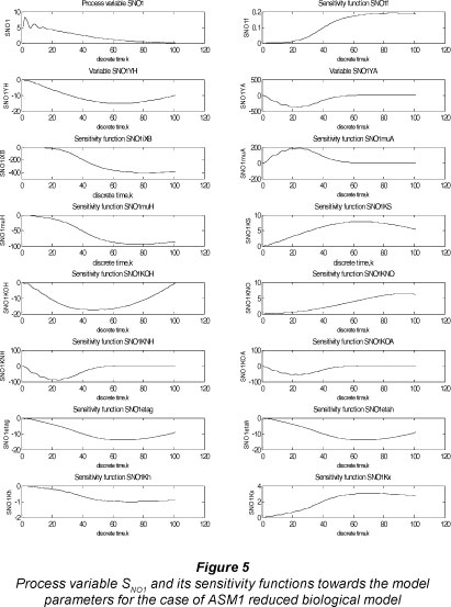
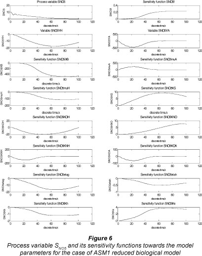
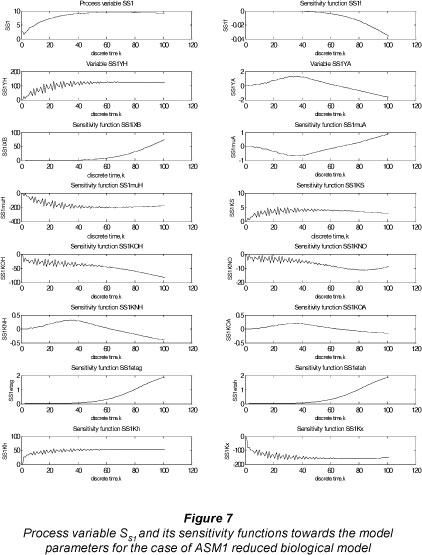
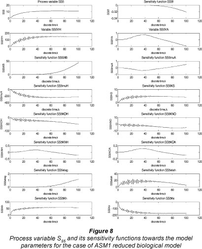
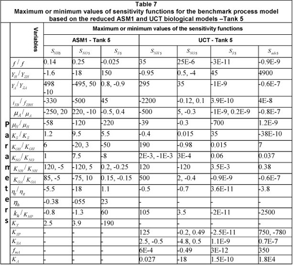
The results from the simulations of the sensitivity functions for Tank 1 and Tank 5 are given in Figs. 3 to 8. The minimum or maximum values of the sensitivity functions are given in Table 6 and Table 7.
Results for the UCT reduced-order biological model
The simulation is done for the parameters given in Table 4 and for the inflow average concentration given by the vector XØ.
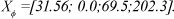
The values for the biomass and the slowly biodegradable substrate are given by the vectors:
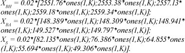
The vector of the dissolved oxygen concentration is:

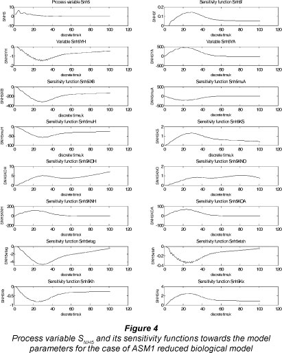
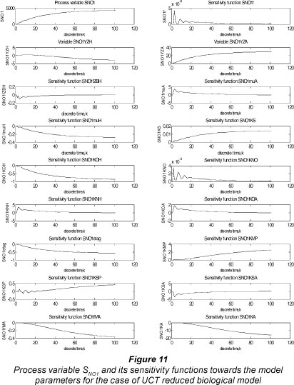
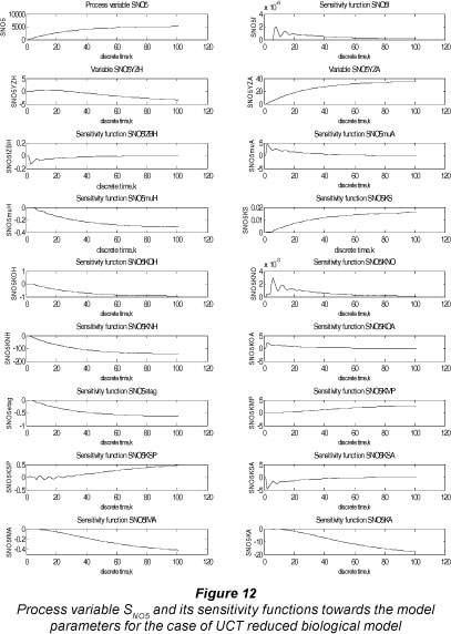
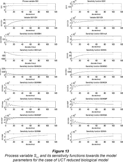
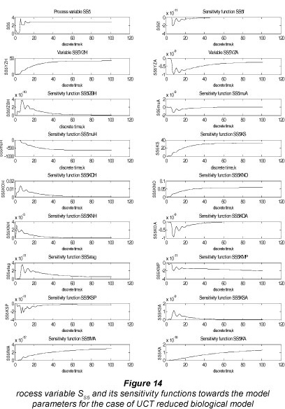
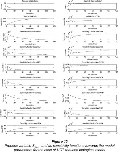
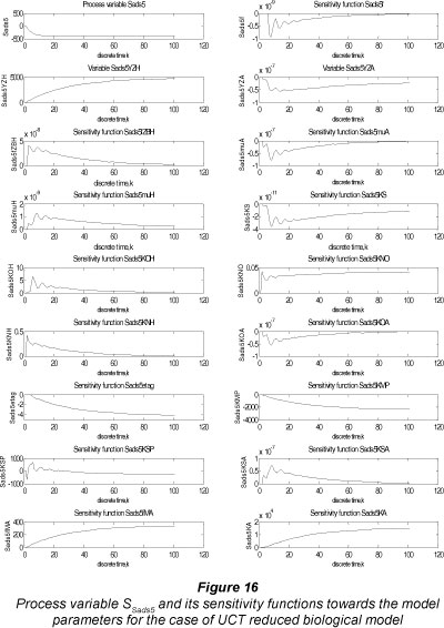
The results from the simulations of the sensitivity functions for Tank 1 and Tank 5 are given in Figs. 9 to 16. The minimum or maximum values of the sensitivity functions are given in Table 6 and Table 7.


Discussion of the results
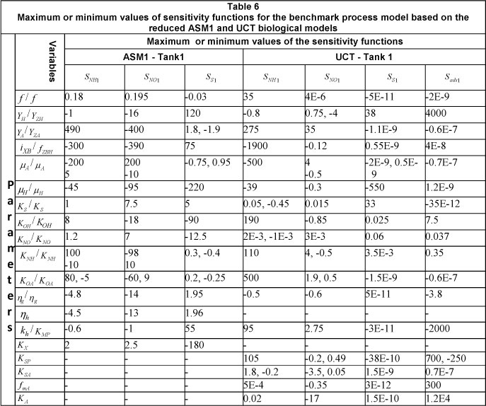
The minimum or maximum values of the sensitivity functions are shown in the tables for the different process variables and parameters. These values can be analysed as follows.
Sensitivity functions simulation for the benchmark process model based on the reduced ASM1 biological model
The sensitivity functions of SNH1 for almost all parameters (without KOH and KNO) display the same type of behaviour. They start from a zero value (in some cases with a small delay), grow in a positive or negative direction to a maximum/minimum value and then reduce to a steady-state value. The maximum/ minimum value is in the time interval between the 5th and 8th hour from the beginning of the simulation period. The steady-state value is achieved at around the 15th hour from the beginning of the simulation period. The maximum values are obtained for parameters f,YA, KS,KOH,KNO,KNH,KOA,KX. The greatest maximum is for parameter YA (490), followed by KNH (100) and KOA (80). The smallest minimums are for parameters iXB (-300), μA (-200), and μH (-45). The behaviour of the sensitivity functions of SNH5 for Tank 5 has the same characteristics as for Tank 1, but the maximum and minimum values of these functions are greater in absolute values, as for example YA (498) and KNH (120) for maximum and iXB (330), μA (-250) and μH (-58) for minimum values. The trajectories of the sensitivity functions are only positive or only negative for most of the parameters. The trajectories for the parameters YA, μA, KNH and KOA develop initially as positive or negative but then at steady-states there is a change in their sign.
The behaviour of the sensitivity functions of the process variable SNOn, n=1, n=5, is similar to that of the variable SNHn, n=1, n=5, but the dynamics of the sensitivity functions are slower, except for parameters YA, μA, KOH KNH and KOA. The maximum or minimum values of the sensitivity functions are reached in a time interval between 15 and 20 h. The maximum sensitivity is towards parameters YA (-400), iXB (-390), μa (200), KNH (-98), μh (-95) and KOA (-60) for the 1st tank, and YA (-495), Íxb (-500), μa (220),KNH(-120), μH (-120) and KOA (-70) for the 5th tank.
The trajectories of the sensitivity functions of the variable SSn, n=1, n=2, are characterised by the slowest dynamics and smallest maximum and minimum values. The maximum values for the 1st tanks are for parameters YH (120), iXB (75), and kh (60), and the minimum values are for parameters μH (-220), KX (-180), and KOH (-90). For the 5th tank the corresponding values are YH (150),iXB(45), kh (60), μh (-220), Kx (-190) and KOH (-50). The maximum and minimum values of the sensitivity functions in this case are for different parameters than those in the 2 vari-ables, SNHn and SNOn considered above.
On the basis of the above it can be concluded that model behaviour is sensitive to parameters YA YH iXB μA KNH μH and KX. The sensitivity of variables SNHn and SNOn, n=1, n=5, is higher than that of variables SSn, n=1, n=5, for parameters YA iXB, μA, and KNH. The sensitivity of the variable SSn, n=1, n=5, is greater for parameters YH, μH, and KX. Some of these parameters can be selected for parameter estimation in order to fit the reduced model to the process data.
Sensitivity function simulation for the benchmark process model based on the reduced UCT biological model
The sensitivity functions of the variable SNHn, n=1, n=5, behave exponentially, with the exception of the sensitivity function for parameter KNO, which displays a small overshoot and then is reduced to a low steady-state value. The steady state maximum/minimum values of the sensitivity functions for the 1st tank are f (35), YZA (275), íxb (-1900), μH (-39), K0h (190), Knh (110), KOA (500),μA (-500), KMP (95), and KSP (105). For the 5th tank the corresponding values are f (35), YZA (295), iXB (-1900), μh(-39), (190), (120), (500), μA (-500), KMP (105), and KSP (125). It can be seen that the sensitivity functions have a time delay and their values are greater for the 5th tank.
For the sensitivity functions of variable SNOn, n=1, n=5, a couple of overshoots at the beginning are then followed by a slow approach to the steady state. The extrema of the sensitivity functions for the parameters are as follows: YZA (35), KNH (4), KSA (-17) for the 1st tank; and YZA (35), KNH (-120), KSA (-18) for the 5th tank. It can be seen that the values of the sensitivity functions in this case are relatively smaller in comparison with the corresponding ones for the first 4 tanks. It is only the influence of parameter KNH which is stronger in the 5th tank.
For variable SSn, n=1, n=5, the sensitivity function displays very low values, and many overshoots for the first 5 hours, with time delays of these trajectories for the 5th tank. After this the trajectories approach steady state. The extrema of the sensitivity functions for the parameters are as follows: YZH (38), μH (-550), and KS (33) for the 1st tank; and YZH (45), μH (-700), and Ks (35) for the 5th tank. The variable SSn, n=1, n=5, is not sensitive to the parameters to which otherprocess variables are sensitive.
The behaviour of the sensitivity functions of variable S , , n=1, n=5, is similar to that for variable Sadsn n=1, n=5. The extrema of the sensitivity functions for the parameters are as follows: YZH (4 000), KOH (7.5), KMP (2 000), KSP (700/-250), fmA (300), and KA (12 000) for the 1st tank, and YZH (4900), KOH (7.5), KMP (2 500), KSP (750/-780), fmA (350), and KA (18 000) for the 5th tank. This variable is very sensitive to the above parameters and extremely insensitive to the rest of the parameters.
Based on the results obtained it can be concluded that the process variables are sensitive to different parameters. Some of these parameters, such as YZH, KMP, KSP, KA, μH, iXB, and KOA, can be selected for estimation in order to fit the reduced model to the process data. The reduced UCT model variables have very low sensitivity to some of the parameters and very high sensitivity to the rest of the parameters. It is difficult to find a group of parameters which result in high values of the sensitivity functions for all variables of the model.
Conclusion
The objective of this study was to describe the development of a sensitivity analysis direct method for developing a reduced model of the activated sludge process, characterised by a large number of parameters and insufficient data measurements. Derivation of sensitivity functions and augmented sensitivity state-space models for the reduced mass balance COST benchmark model, based on reduced ASM1 and UCT biological models, was presented. Matlab software was developed and simulations provided. The results enable one to answer the question as to which of the parameters need to be estimated in order to fit the reduced model behaviour to the data. Selection of the candidate parameters for estimation was based on a comparison of the minimum or maximum values of the corresponding sensitivity functions. The shapes of the sensitivity functions obtained for all variables and parameters of Tank 1 for the benchmark process model, based on the reduced ASM1 or reduced UCT biological models, are similar to the corresponding functions for Tank 5. The difference is in the minimum or maximum values of the sensitivity functions, which are greater for Tank 5 . Another difference is that the sensitivity function trajectories for the 5th tank have a time delay and are slower. Different combinations of parameters selected by the sensitivity analysis were estimated and the trajectories of the estimated model showed a good fit to the measured data. The methods used, algorithms, Matlab software and results for parameter estimation are not discussed in this paper. The reduced models, if properly calibrated, can predict the process behaviour, with small errors. These models are usually developed for real-time control design as a response to inflow disturbances. Reduced model applications for detailed studies of process interaction between variables, kinetic parameters and output performance will not be as successful as the application of the full models.
The main contribution of the study reported herein is that it provides a quantitative basis for classification of the model parameters. This helps to address the problems of complexity and uncertainty during the process of parameter estimation for nonlinear models. The proposed structure of the augmented sensitivity model is general and modular which permits its application to any wastewater treatment process and to any other nonlinear model. The vector/matrix structure of the model allows effective use of Matlab software and rapid solution of the simulation sensitivity problem. This means that the proposed structure of the augmented model assures global sensitivity analysis without increasing the computation burden.
The developed algorithms and software can be used for different applications: to simplify models, to investigate robustness of the proposed parameter estimation results, to analyse different scenarios for the plant operation, to determine the region of the parameter space for which the output is minimum or maximum, to discover interactions between the input factors (variables and parameters), to discover issues not anticipated at the beginning of the investigation, and to use in real-time joint solution of the problem of parameter estimation, control design and implementation, as a part of an adaptive control strategy.
Acknowledgements
This study was funded by KISC NRF Grant No. 63667 'Coordinated and joint research activities in wastewater treatment monitoring, modelling, estimation and control in real-time'."
References
AL-SAGGAF UM and FRANKLIN GF (1988) Model reduction via balanced realizations: an extension and frequency weighting techniques. IEEE Trans. Autom. Control AC-33 (7) 687-692. [ Links ]
BECK C, DOYLE J AND GLOVER K (1996) Model reduction of multi-dimensional and uncertain systems. IEEE Trans. Autom. Control 41 (10) 1466-1477. [ Links ]
BREYFOGLE FW III (2003) Implementing Six Sigma: Smart Solution using Statistical Methods (2nd edn.). John Wiley and Sons, New York. [ Links ]
COPP J (2002) COST Action 624 - The Cost Simulation Benchmark: Description and Simulation Manual. Office for Official Publications of the European Union, Luxembourg. [ Links ]
DE PAUW D and VANROLLEGHEM P (2003) Practical aspects of sensitivity analysis for dynamic models. URL: http://www.bio-math.rug.ac.be. (Accessed 12 June 2009). [ Links ]
DOCHAIN D (2003) State and parameter estimation in the chemical and biochemical processes: a tutorial. J. Process Control 13 801-818. [ Links ]
DOLD P, EKAMA G and MARAIS G (1980) A general model for the activated sludge process. Prog. Water Technol. 12 47-77. [ Links ]
DU PLESSIS SC (2009) The investigation of the process parameters and developing a mathematical model for purposes of control design and implementation of the wastewater treatment process. D.Tech. thesis, Cape Peninsula University of Technology, Cape Town. [ Links ]
EKAMA G, MARAIS G, PITMAN A, KEAY, G, BUCHAN L, GERBER A and SMOLLEN M (1984) Theory, Design and Operation of Nutrient Removal Activated Sludge Process. WRC Report No. TT 16/84. Water Research Commission, Pretoria. [ Links ]
EKAMA G and MARAIS G (1979) Dynamic behaviour of the activated sludge process. J. Water Pollut. Control Fed. 51 534-556. [ Links ]
FESSO A (2007) Statistical sensitivity analysis and water quality. In: Wymer I (ed.) Statistical Framework for Water Quality Criteria and Monitoring. Wiley, New York. [ Links ]
FRANK P (1978) Introduction to System Sensitivity Theory. Academic Press, London. [ Links ]
GLOVER K (1984) All optimal Hankel-norm approximations of linear multivariable systems and their L∞ error bounds. Int. J. Control 39 (6) 1115-1193. [ Links ]
HALEVI Y, ZLOCHEVSKY A and GILAT T (1997) Parameter-dependent model order reduction. Int. J. Control 66 (3) 463-485. [ Links ]
HENZE M, GRADY J, GUJER W, MARAIS G and MATSUO T (1987) Activated sludge model No. 1.1AWPRC Scientific and Technical Report No. 1, IAWPRC task group on mathematical modeling for design and operation of biological wastewater treat-ment, London. [ Links ]
HOLMBERG A and RANTA J (1982) Procedures for parameter and state estimation of microbial growth process models. Automatica 18 181-193. [ Links ]
JEPPSSON U (1996) Modeling Aspects of Wastewater Treatment Processes. Thesis, Lund University, Lund, Sweden. [ Links ]
LATHAM A and ANDERSON BDO (1985) Frequency-weighted optimal Hankel-norm approximation of stable transfer functions. Syst. Control Lett. 5 229-236. [ Links ]
LENNOX B, MONTAGUE GA, HIDEN HG, KORNFELD G and GOULDING PR (2001) Process monitoring of industrial fed-batch fermentation. Biotechnol. Bioeng. 74 (2) 125-135. [ Links ]
LOURIES A, ZCELY, CSIKOSZ-NAGY, TURANYI T and NOVAK B (2008) Analysis of a budding yeast cell cycle model using the shapes of local sensitivity functions. Int. J. of Chem. Kinet. 40 (11) 710-720. [ Links ]
MONTGOMERY DC (1997) The Use of Statistical Process Control and Design of Experiments in Product and Process Improvement. IIE Trans. 24 479. [ Links ]
MOORE BC (1981) Principal component analysis in linear system: Controllability, observability and model reduction. IEEE Trans. Autom. Control AC-26 17-32. [ Links ]
MUSSATI M, GERNAEY K, GANI R and J0RGENSEN S (2002) Computer aided model analysis and dynamic simulation of a waste-water treatment plant. Clean Technol. Environ Polic. 4 100-114. [ Links ]
NOYKOVA N and GYLLENBERG M (2000) Sensitivity analysis and parameter estimation in a model of anaerobic waste water treatment processes with substrate inhibition. Bioprocess Eng. 23 343-349. [ Links ]
PERTEV C, TURKER M and BERBER R (1997) Dynamic modeling, sensitivity analysis and parameter estimation of industrial yeast fermenters. Comp. Chem. Eng. 21 739-744. [ Links ]
PLAZL I, PIPUS G, DROLKA M, and KOLOINI T (1999) Parametric sensitivity and evaluation of a dynamic model for Single-stage wastewater treatment plant. Acta Chim. Slov. 46 (2) 289-300. [ Links ]
SAFANOV MG and CHIANG RY (1989) A Schur method for balanced-truncation method reduction. IEEEAutom. Control AC-34 729-733. [ Links ]
SATO J and OHMORI H (2002) Sensitivity analysis and parameter identification of wastewater treatment based on Activated Sludge Model No. 1 (ASM 1). Proceedings of SICE 2002, 5-7 August 2002, Osaka. 434-439. [ Links ]
SCHERMANN PS and GARAG-GABIN W (2005) Process Gain, Time Lags and Reaction Curves. In: Liptak BG (ed.) Instrument Engineer's Handbook: Process Control and Optimization. Pergamon Press, New York. [ Links ]
SMETS I, BERNAERTS K, SUN J, MARCHAL K, VANDER-LEYDEN J and VAN IMPE J (2002) Sensitivity function-based model reduction. A bacterial gene expression case study. Biotech. Bioeng. 80 195-200. [ Links ]
STECHA J, CEPAK M, PEKAR J and PACHNER D (2005) System Parameter estimation using p-norm minimization. Preprints from Proceedings of the 16th IFAC World Congress, 4-8 July 2005, Prague, Czech Republic. [ Links ]
TSONEVA R, POPCHEV I and PATARINSKA T (1996) Minimum time sensitive control of nonlinear time delay systems with slowly varying parameters. Proc. 13th IFAC World Congress, 1 April 1997, San Francisco. E 371-376. [ Links ]
VARMA A, MORBIDELLI M and WU H (1999) Parametric Sensitivity in Chemical Systems. Cambridge University Press, Cambridge. [ Links ]
WANG L and GAWTHROP PJ (2001) On the estimation of continuous time transfer functions. Int. J. Control 74 889-904. [ Links ]
WENTZEL M, EKAMA G and MARAIS G (1992) Processes and modelling of nitrification, denitrification and biological excess phosphorus removal systems. Water Sci. Technol. 25 (6) 59-82. [ Links ]
WISNEWSKI PA and DOYLE III FJ (1996) A reduced model approach to estimation and control of a Kamyr digester. Comput. Chem. Eng. 20 1053-1058. [ Links ]
Received 7 August 2009;
Accepted in revised form 2 April 2012.
* To whom all correspondence should be addressed. +27 21 959-6459; fax: +27 21 959-6117 E-mail: tzonevar@cput.ac.za


