


Services on Demand
Article
 English (pdf)
 Article in xml format
 Article references
Indicators

Related links
-
 Cited by Google
 -
 Similars in Google
Share

 Permalink
Water SA
On-line version ISSN 1816-7950
Print version ISSN 0378-4738
Water SA vol.38 n.2 Pretoria Jan. 2012
ARTICLES
Synthetic monthly flow duration curves for the Cape Floristic Region, South Africa
Allen Hope*; Ryan Bart
Department of Geography, San Diego State University, San Diego, CA 92182, USA
ABSTRACT
A flow duration curve (FDC) provides a valuable planning and management tool since it describes the entire flow regime of a river. Water resource planning in South Africa is often based on monthly river flow data and synthetic FDCs are required for applications in ungauged catchments. The objective of this study was to derive 11 monthly FDC percentile flows and the mean annual flow (MAQ) for catchments in the Cape Floristic Region of South Africa using regression equations with readily measureable catchment variables, including vegetation indices from Moderate Resolution Imaging Spectrometer (MODIS) satellite imagery. An 'all-models' approach with 10-fold validation was adopted to identify the 'best' regression models. Predictions of percentile flows above the median flow and MAQ were generally good but poor for low flows. Overall predictive uncertainty had a tendency to be larger in drier catchments. The most important predictive variables were catchment mean annual precipitation, physiography and soils. MODIS vegetation indices were significant predictors in equations for 6 percentile flows and MAQ, and predictive uncertainty increased if the MODIS indices were excluded from model development. The regression approach implemented in this study may be appropriate for other regionalisation studies that are based on a small sample of gauged catchments.
Keywords: Western Cape Region, flow duration curve, ungauged catchments, multiple regression, cross-validation
Introduction
A flow duration curve (FDC) is a graphical representation of the frequency distribution of the complete river flow regime and is one of the most commonly-used techniques in hydrology (Croker et al., 2003). While empirical FDCs can be developed using gauged flow data, estimation of FDCs in ungauged catchments requires a regionalisation approach which is usually based on flow information from a network of gauged sites. The International Association of Hydrological Sciences (IAHS) Decade on Predictions in Ungauged Basins (PUB) is an international initiative that recognises the critical need to advance hydrological predictions in ungauged catchments (Sivapalan, 2003). River flow prediction in ungauged catchments is widely regarded as the ultimate challenge in hydrology (Sivapalan, 2003).
A number of regionalisation approaches have been proposed for estimating FDCs in ungauged catchments. A common regionalisation methodology describes the FDC in terms of a mathematical model and then relates the parameters of the model to catchment morphological and/or climatic variables using regression analysis (Niadas, 2005; Viola et al., 2011). Probabilistic models can be used to describe the FDC and regression models developed to estimate the parameters of the distribution (Castellarin et al., 2007)
Assumptions regarding models that describe the form of FDCs can be avoided by developing regional regression equations to predict the selected percentile flows (e.g., flows for exceedance percentages 5%, 10%, 20%, ...95%). Catchment physical characteristics are used as the predictor variables in these regression equations (e.g., Mohamoud, 2008; Yu and Yang, 2000). This approach has been used successfully by Yu and Yang (2000) in Taiwan to predict daily stream flow for 10 percentile flows in ungauged catchments. Precipitation was largely uniform across the study region and catchment area was the only independent variable in all 10 linear regression equations. Predictions of low-flow discharge (80% and 90% exceedance probabilities) were less accurate than those for the higher flows (Yu and Yang, 2000). A similar regionalisation scheme to predict FDCs in the United States Mid-Atlantic Region was developed by Mohamoud (2008). In contrast to the study conducted by Yu and Yang (2000), a comprehensive set of catchment descriptors (n = 42) were investigated as potential independent variables in the percentile flow regression equations. These variables represented catchment land use/land cover, geomorphology, geology and climate and a step-wise regression approach was used to select the best predictor variables (Mohamoud, 2008).
A major impediment to the development of FDC region-alisation schemes relates to the number of gauged rivers in a region. Small sample sizes impact the reliability of equations to predict FDCs and restrict the number of variables that can be used in the equations. While this is a problem in many developed countries, the problem is generally more acute in developing countries where limited resources preclude installing and maintaining extensive gauging networks. Despite this limitation, the pressing need for flow information in ungauged catchments requires that attempts be made to formulate regionalisation schemes using available flow data.
Water resource development and management decisions in South Africa are usually based on monthly stream flow characteristics (Hughes and Smakhtin, 1996; Smakhtin, 2001). Laws and policies have been implemented in South Africa that give priority of water to ecosystems once basic human needs have been met (Acreman and Dunbar, 2004). The term 'environmental flows' refers to a flow regime which will maintain a river in some specified condition (Smakhtin, 2007). In many countries, the concept of minimum flow level was the initial focus for establishing environmental flows, but now it is increasingly recognised that all elements of a flow regime are important to manage river ecosystems (Acreman and Dunbar, 2004).
There is a need for rapid, low-confidence hydrological predictions in South African catchments to facilitate initial planning related to ecological instream flow requirements (Hughes and Hannart, 2003). Synthetic FDCs facilitate planning activities in ungauged catchments and have become an integral part of environmental flow assessments (Smakhtin, 2007). This study was initiated to investigate the feasibility of developing a FDC regionalisation scheme for a critical ecological and economic region of South Africa, the Cape Floristic Region (CFR). The CFR has a Mediterranean-type climate (wet winters and dry summers) with catchments that are physi-ographically and hydromorphometrically distinct from catchments in the summer precipitation region of South Africa (Seyhan and Hope, 1983). The dominant natural vegetation is a schlerophyllous shrubland (fynbos) and is home to over 9 000 plant species, including the highest known concentration of rare species in the world (Cowling and Hilton-Taylor, 1994; Rouget et al., 2003). The CFR includes the Cape Town metropolitan area which is dependent on local rivers for most of its water supply. Catchments in the CFR are under pressure from agricultural development, diminished stream flow associated with invasion by exotic plant species and rapid urbanisation (Rouget et al., 2003). These catchments require careful management to ensure flows can sustain both riparian and estuarine aquatic ecosystems.
The specific aim of this study was to develop a monthly FDC regionalisation scheme for small and intermediate size catchments (area < 300 km2) in the CFR. Larger catchments were excluded since they are more prone to having dams, development and water abstractions than smaller catchments, and to avoid excessive intra-catchment heterogeneity. Recognising that the number of gauged catchments for the investigation was likely to be small, a goal was to design and implement a rigorous regression approach to predict percentile flows. Since data and vegetation indices (e.g., leaf area index, spectral vegetation indices) from the Moderate Resolution Imaging Spectrometer (MODIS) satellite imagery are readily available, a secondary objective was to test the utility of MODIS vegetation indices for predicting FDC percentile flows.
Methods
Study region and catchments
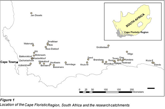
The CFR covers 87 892 km2 (Fig. 1) and while it is characterised by a Mediterranean-type climate, a limited amount of precipitation occurs during the summer months; increasing from west to east across the region (Goldblatt and Manning, 2002). Mean annual precipitation (MAP) ranges from 200 mm in the western lowlands to 3 600 mm in the high mountains (Linder, 1991). Free water evaporation is between 1 250 and 1 600 mm/yr (Seyhan and Hope, 1983). The region is characterised by diverse physiography which includes sandy coastal plains underlain by shale; low mountains of limestone, sandstone and conglomerate; undulating hills underlain by shale located along the inland margins of the coastal plains; and rugged mountain ranges comprised primarily of sandstones that rise abruptly to 2 000 m (Goldblatt and Manning, 2002). As mentioned earlier, the shrubland landscapes of the CFR are characterised by remarkably high species richness (Linder, 1991; Cowling and Hilton-Taylor, 1994; Rouget et al., 2003). Forests tend to be located in areas of deeper soils and high precipitation while most of the hills and valleys are under agriculture (Linder, 1991).
River flow data were obtained from the South African Department Water Affairs (DWA). All gauged rivers in this region with catchment areas of less than 300 km2 were identified as potential candidates for the study. Larger catchments were excluded in this proof-of-concept study since they are more prone to having dams, development and water abstractions than smaller catchments. A set of elimination criteria were applied to identify the final set of study catchments and to minimise uncertainties in the derivation of percentile flows. Catchments were required to have a minimum of 10 years of high quality river flow record. In a FDC regionalisation study in Italy, Castellarin et al. (2007) concluded that 5 years of observed river flow data was sufficient to obtain consistent estimates of the long-term FDC. Catchments with impoundments (e.g., dams), water diversions, and significant urbanisation or agriculture (>5% of catchment area) were excluded and it was assumed that no major changes in land-cover occurred during the period of investigation.
Catchment variables
From an initial pool of 125 catchments, 30 were found to be suitable for the investigation. Characteristics of these catchments are summarised in Table 1 and their locations in the CFR are indicated in Fig. 1. This small sample size is not unusual for regionalisation studies such as those conducted by Yu and Yang (2000) in southern Taiwan (n = 10) and Mohamoud (2008) in the Mid-Atlantic Region, USA (n = 29). Monthly river flow was expressed as a depth and period-of-record FDCs were constructed for each catchment. These FDCs were used to determine 11 percentile flows for regionalisation (i.e., Q5, Q10, Q20, Q30, Q40, Q50, Q60, Q70, Q80, Q90 and Q95).
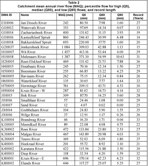
The river flow characteristics and record length for the 30 study catchments are summarised in Table 2. The catchment sample covered a wide range of wetness conditions, with mean annual river flow (MAQ) ranging from 12 mm for the Sand River to 1 457 mm for the Wit River (Table 2). Percentile flows for high (Q5), medium (Q50) and low (Q95) flows in Table 2 also indicate a good distribution of flow regimes in the selected catchments and two of the rivers (Sand and Smalblaar) are ephemeral.
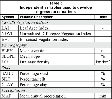
Catchment variables characterising vegetation, physiography, soils and precipitation were tested as independent variables in regional regression equations to predict percentile flows and MAQ. Vegetation descriptors were based on MODIS satellite data from the Terra satellite which was launched by the US National Aeronautics and Space Administration (NASA) in 1999. These data are converted on a systematic basis into derived terrestrial products, including indices that quantify vegetation cover (Justice et al., 2002). The USGS Land Processes (LP) Distributed Active Archive Center (DAAC) at the Earth Resources Observation and Science (EROS) Data Center distributes these MODIS products. Three MODIS vegetation products were used in the study - 2 spectral vegetation indices and leaf area index (LAI). The 2 spectral vegetation indices were the Normalised Difference Vegetation Index (NDVI) and the Enhanced Vegetation Index (EVI). These indices are obtained from:

where:
p is surface red or near infrared (nir) reflectance (Tucker, 1979), and
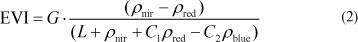
where:
G is a gain factor
L is a canopy background adjustment term (addresses non- linearity of radiation transfer)
ρblue is the surface blue reflectance
C1 and C2 are weights to correct for different atmospheric aerosol concentrations (Huete et al., 2002)
The EVI is intended to be less sensitive to variations in atmospheric conditions than the NDVI and to have a lesser tendency to saturate at high LAI values (Guo et al., 2007). LAI is estimated by inversion of a radiative transfer model which uses MODIS spectral reflectance data (Myneni et al., 2002).
The NDVI, EVI, and LAI products for the study area were obtained from the EROS Data Center DAAC for a regional study funded by the United States National Aeronautics and Space Administration (Hope et al., 2005) and covered the period April 2000 through March 2006. The data have a ground resolution of 1 km and values are provided at 16-day intervals for NDVI and EVI and every 8 days for LAI. Average NDVI, EVI, and LAI values were calculated for each catchment over the 6-year period.
Three physiographic variables were calculated for each catchment using a 90 m digital elevation model for the region that was developed using data from the Shuttle Radar Topographic Mission (SRTM) and provided by the South African Agricultural Research Council, Institute for Soil Climate and Water (ARC-ISCW). These physiographic variables were mean elevation, mean slope and drainage density. Data from ARC-ISWC were used to determine the average fraction of sand, silt and clay for soils in the catchments. MAP was obtained from 1-km gridded precipitation data also provided by the ARC-ISCW. Gridded values were based on interpolating data from all available precipitation gauges in the region and included an adjustment for elevation (J. Malherbe, 2006). The list of independent variables with their abbreviations and units of measurement are given in Table 3.
Regression models
Multiple regression models may be developed to produce the single 'best' model for prediction or to infer causal influences of selected independent variables on the dependent variable (Mac Nally, 2000). Stepwise regression techniques are often used to identify predictive models, but there is wide recognition that this is a flawed approach that is likely to yield spurious results (Mac Nally, 2000). The technique frequently does not choose the best model predictors and is prone to producing inflated coefficient of determination values (R2), leading to poor model performance in validation (Keith, 2006).
Given current computer power, it is now generally feasible to conduct an exhaustive search of all possible independent variable combinations ('all-models') to identify the best model (Mac Nally, 2000). Model selection criteria need to be defined to provide a compromise between model 'fit' and model 'com-plexity' (Mac Nally, 2000). Model fit is usually evaluated by an objective function based on the residual sum of squares while model complexity is indicated by the number of model terms.
The all-models approach was adopted in this study with a set of catchment descriptors (independent variables) to identify the best predictive models for the 11 percentile flows and MAQ. Additive and multiplicative model structures were tested along with an exhaustive search using untransformed and log-transformed variables to allow for linear and nonlinear relationships between dependent and independent variables (Berger, 2004). Given the sample size for model development (n = 30), model complexity was limited to 4 terms. A 2-step strategy was implemented to select the best model for each level of complexity. The first step screened all models for multicolinearity and the remaining models were then ranked according to their adjusted R2 to identify the best model. Adjusted R2 is a modified version of R2 which decreases the R2 value based on the number of explanatory terms in the model.
The degree of multi-colinearity was quantified in Step 1 using the condition index (CI) which is given by:

where:
for a given set of independent variables, λ are the eigenvalues of the rescaled crossproduct X'X matrix (Belsley et al., 1980).
The index value increases with increasing colinearity and, since the index is considered situational, only rules of thumb exist to reject models. Models with CI greater than 15 were rejected since Belsley et al. (1980) suggest that weak dependencies are associated with CI values around 5 or 10 and strong relations are associated with values above 30.
The selection of the best model structure at each percentile flow from the 4 calibrated models (1 to 4 terms) depends on how well the models predict percentile flows in 'ungauged' or validation catchments. Unfortunately, a small sample size is often the reality investigators have to face when they conduct regionalisation studies using gauged catchment data. The challenge for regression analyses is to have an adequate sample for model development and validation. The holdout method, which splits the samples into independent calibration and validation datasets, is hindered by an inefficient use of sample data in the calibration model which increases prediction bias (Kohavi, 1995; Blum et al., 1999). A cross-validation approach, such as the k-fold technique (Kohavi, 1995), can be used to sample all of the data during calibration when it is not practical to withhold a sub-set for validation.
The k-fold validation technique divides the sample data evenly into k groups or folds, which are then systematically removed from the calibration data as a validation set. This process is repeated k times, and when k equals the number of samples in the data the technique is commonly referred to as a jackknife. Breiman and Spector (1992) and Kohavi (1995) recommend the use of a 10-fold cross-validation. Although predictions using the 10-fold cross-validation are generally more biased than in the jackknife approach, prediction variance is considerably reduced, leading to more accurate estimations and better results than the jackknife approach (Kohavi, 1995).
For each regression model (1 to 4 terms) developed using all catchments in calibration, we used a 10-fold cross-validation with the removal of 3 catchments during each resample. The 3 catchments were selected by stratified random sampling, with 3 strata defined by magnitude of the percentile flow (3 equal class widths). A random catchment was selected from the upper-, middle- and lower-flow class for model validation. Observed and predicted flow values for the 3 validation catchments from all of the 10-folds were then pooled to evaluate the validation performance of each model. The Nash and Sutcliffe (1970) coefficient of efficiency (NSE) was calculated from the observed and estimated flow values to quantify the validation performance of the 4 models tested for each percentile flow (i.e., a measure of the overall agreement between observed and predicted flow values for the validation catchments). The NSE is the ratio of model error variance to the variance of observed values, subtracted from 1.0. This index was used by Castellarin et al. (2004) to compare modelled and observed per-centile flows and they considered values above 0.75 to indicate 'good' agreement.
The single best model for each percentile flow was selected from the 4 models (1 to 4 terms) using the largest NSE values determined from the 10-fold validation. We calculated the relative root-mean-square-error (RRMSE) for each of these regional models to assess the magnitude of predictive uncertainty. The RRMSE is the root-mean-square-error divided by the average percentile flow for all catchments.
Contribution of MODIS variables
The regression approach outlined above was repeated with the 3 MODIS variables excluded from the pool of potential predictor variables. Validation results (NSE, RRMSE) from both analyses were compared to assess how these variables affected predictive uncertainty. We also compared the relative performance of the predictive equations in each catchment using 'relative error' (RE) as suggested by Castellarin et al. (2004) and referred to as BIAS by Croker et al (2003). This quantity is obtained from:
where:
QE and Q0 are respectively estimated and observed percen-tile flows (or MAQ).
For each catchment, we summed the absolute RE values from each predictive equation used in validation to quantify the overall uncertainty in the estimated FDC.
Results and discussion
Model selection and validation
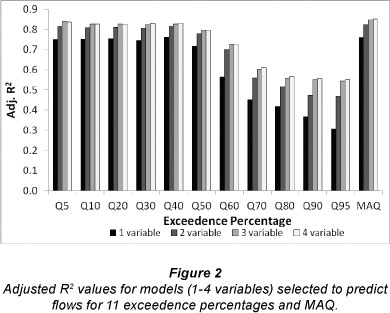
Adjusted R2 values for the 4 best models (1 to 4 variable models) to predict percentile flows and MAQ are displayed in Fig. 2. In most cases, inclusion of more independent variables increased the adjusted R2 even though this statistic adjusts for the number of independent variables. Models for the higher flows (Q5 - Q50) were better than those for the flows below Q60, with the best adjusted R2 values all greater than 0.8 (Fig. 2). The 1-term models had substantially smaller adjusted R2 values than the other models while there was little difference in the adjusted R2 of the 3- and 4-term models.
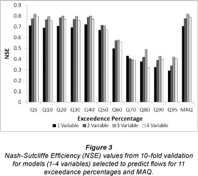
The NSE values obtained using 10-fold validation of the best models are given in Fig. 3. As expected from the model development results, prediction of percentile flows above Q60 were notably better than predictions for the low flows (Fig. 3). However, the model performance did not improve consistently with the number of variables included in the equations as was the case in the model development phase. Models with 4 variables were not the best models in validation for any of the percentile flows or MAQ (Fig. 3). Instead, models with 3 variables were the best models in validation except for Q50 (2 variables) and Q70 (1 variable). Only equations for percen-tile flows above Q50 and for MAQ had NSE values greater than 0.75, the threshold suggested by Castellarin et al. (2004) to indicate 'good' FDC models.
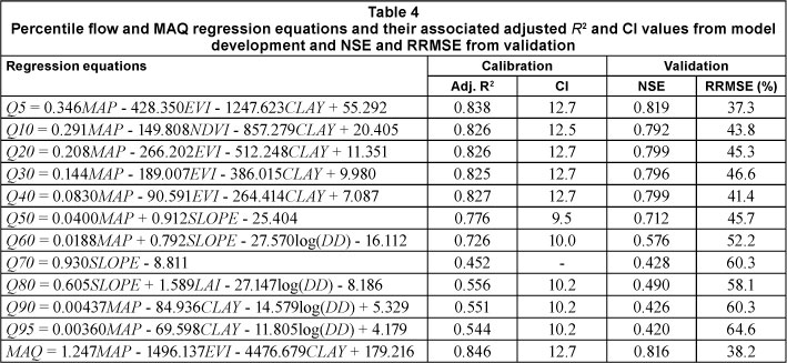
The best regression models for each percentile flow and MAQ based on validation performance are given in Table 4 along with their adjusted R2 and CI values from model development and the validation statistics (NSE, RRMSE). In all cases, additive models were selected over the multiplicative models. Models for percentile flows from Q5 to Q50 and for Q70 and MAQ were linear while the remaining models for low flows included logarithmic terms (Table 4). All models included MAP except the Q70 and Q80 models, while soil clay fraction (CLAY) appeared in the high-flow models and in the MAQ and Q95 models. Although the adjusted R2 and NSE values from model development and validation were greater than 0.7 for percentile flows Q5 to Q50, validation RRMSE values were all greater than 37% (Table 4), indicating potentially large uncertainty in predicting these quantities in ungauged catchments.
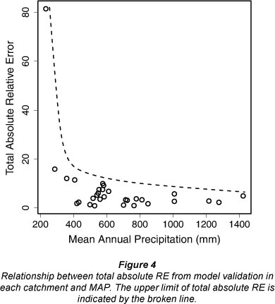
Since the prediction of low flows was found to be uncer-tain, it seemed likely that the overall regionalisation approach may be better suited to wet, rather than dry catchments. For each catchment, we summed the absolute RE values from each predictive equation used in validation and then plotted this total RE against MAP (Fig. 4). The upper limit of total RE in Fig. 4 (broken line) increased as MAP decreased, indicating the potential for larger uncertainties in the drier catchments. The total absolute RE for the driest catchment (Sand River) was considerably larger than values in the other catchments, indicating a possible threshold MAP (less than 300 mm) for appropriate use of this approach. These findings are similar to those reported by Yu and Yang (2000) and Hope and Bart (2012), who also found weaker models for predicting the low percentile flows for FDCs in Taiwan and southern California USA, respectively. In each of these studies, processes controlling low flows may not have been adequately represented by the variables used in the models or uncertainties in the measurement of low flows may have contributed to predictive errors.
Effect of MODIS variables
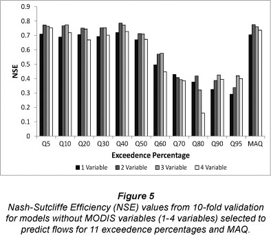
When MODIS variables were included in the development phase of the flow prediction models, 7 of the 12 equations included these variables (Table 4). The EVI was included in equations for Q5, Q20, Q30, Q40 and MAQ while the NDVI was in the equation for Q10 and LAI was selected for the Q80 model. The 10-fold validation results (NSE, RRMSE) given in Fig. 5 are for equations developed with MODIS variables excluded from the model development phase. All NSE values in Fig. 5 were smaller than values for corresponding models that did include MODIS variables (Fig. 3).
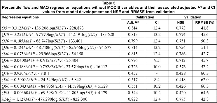
The best regression models without MODIS variables that were identified using the 10-fold validation are given in Table 5. While models to predict percentile flows that included MODIS variables (Table 4) had better calibration results than models without MODIS variables (Table 5), the differences in NSE and RRMSE were not substantial. At most, the RRMSE was 5% smaller with MODIS variables in the equations. Except for Q70 and Q80, catchment MAP was the first variable to enter the regression equations, reflecting the dominant effect of this variable for the estimation of percentile flows and MAQ. While these results appear to indicate that vegetation has a small effect on river flows, the results also may be a consequence of the research methodology. The vegetation indices were represented in the regression equations as area- and time-averaged values for each catchment. Vegetation effects on hydrological fluxes in different parts of the catchments and at different times of the year could not be represented. For example, transpiration associated with phreatophytic vegetation located within the 0.9 0.8 0.7 0.6 0.5 0.4 0.3 0.2 0.10 riparian zone could be expected to impact low flows more than transpiration from vegetation on the hill slopes. This was demonstrated by Hope et al. (2009), who found a significant relationship between a spectral vegetation index (NDVI) in the lowland area of a CFR catchment (Molenaars) and annual flow volume, but no relationship when the index was calculated for the upland areas.
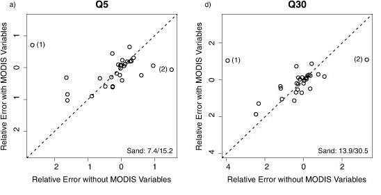
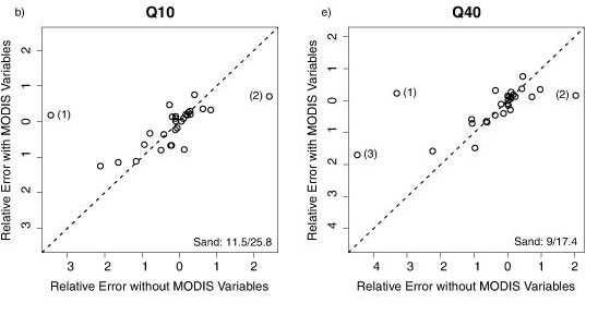
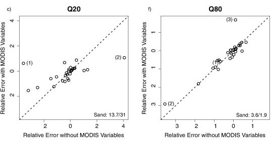
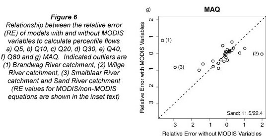
To assess the effect of MODIS variables on the prediction of percentile flows in individual catchments, the average RE values from validation of models with and without MODIS variables were plotted against each other (Figs. 6a-6g). The exclusion of MODIS variables from the predictive equations had little effect on predictive accuracy in most catchments, with most of the points plotting around the 1:1 lines (Fig. 6). However, in 3 catchments (Sand River, Brandwag River and Wilge River) the exclusion of MODIS variables caused large predictive errors for percentile flows Q5-Q40 and MAQ (Fig. 6). Prediction errors in the Smalblaar River catchment were also notably larger for models without MODIS variables to predict Q40 (Fig. 6e) and MAQ (Fig. 6g), but smaller to predict Q80 (Fig. 6f). These 4 catchments (Sand, Brandwag, Wilge and Smalblaar Rivers) are also the catchments with the 4 lowest mean annual flows (MAQ) (Table 2). Since soil moisture rather than the amount of vegetation tends to be the controlling variable affecting evaporative losses and river flow in water-limited catchments, it is not apparent why vegetation indices were more important variables in these drier catchments than in wetter catchments. However, given the small sample of catchments used in this study, direct conclusions regarding the effect of vegetation on river flows may not be appropriate.
Conclusion
A goal of this study was to develop regional regression equations that could be used to predict monthly FDC percentile flows and MAQ from readily measureable catchment variables, including satellite-derived vegetation indices. The all-models approach with 10-fold validation was found to be suitable for use with the restricted catchment sample size available for this study. The challenge of predicting low flows in semi-arid catchments is well documented (e.g., Pilgrim et al., 1988; Croke and Jakeman, 2008) and, as expected, the prediction of the larger percentile flows (Q5 - Q50) and MAQ were notably better than prediction of low flows. Based on the prediction equations for FDC percentile flows in the CFR, it may be concluded that catchment mean annual precipitation, physiography and soils were more important predictive variables than MODIS vegetation indices. Use of MODIS vegetation variables in the regression equations did not result in substantially better calibration results in most catchments, but did reduce predictive uncertainty substantially in 3 or 4 catchments depending on the flow calculation.
While the validation results of this study pointed to large uncertainties in the prediction of percentile flows, the set of equations provide a means for rapid, low-confidence estimates for initial catchment planning, as suggested by Hughes and Hannart (2003). Uncertainties in the measurement of river flows, due to flows exceeding the available rating curves and the possibility that some low flows were impacted by undocumented abstractions, may have contributed to prediction uncertainties. More reliable synthetic FDCs may be attainable if a larger sample of study catchments could be identified. Alternative approaches should also be investigated where regression equations are used to derive parameters of mathematical or probabilistic FDC models (e.g., Niadas, 2005; Castellarin et al., 2007).
Acknowledgements
Assistance with data processing and the construction of the tables and figures was provided by Noah Albers and Keith James (San Diego State University). We gratefully acknowledge the assistance with data sets provided by the Agricultural Research Council, Institute for Soil Climate and Water (Terrence Newby, Talita Germishuyse, Johan Malherbe and Ian Kotze). This study was funded by the U.S. National Aeronautics and Space Administration, Land Cover Land Use Change Program, Grant No. NNG05GR14G.
References
ACREMAN M and DUNBAR MJ (2004) Defining environmental river flow requirements - a review. Hydrol. Earth Syst. Sci. 8 861-876. [ Links ]
BELSLEY DA, KUH E and WELSCH RE (1980) Regression Diagnostics. John Wiley and Sons, New York. [ Links ]
BERGER DE (2004) Using regression analysis. In: Wholey JS, Hatry HP and Newcomer KE (eds.) Handbook of Practical Program Evaluation. Wiley, San Francisco. 479-505. [ Links ]
BLUM A, KALAI A and LANGFORD J (1999) Beating the hold-out: bounds for K-fold and progressive cross-validation. In: COLT '99 Proceedings of the Twelfth Annual Conference on Computational Learning Theory. ACM, New York. 203-208. [ Links ]
BREIMAN L and SPECTOR P (1992) Submodel selection and evaluation in regression. The X-random case. Int. Stat. Rev. 60 291-319. [ Links ]
CASTELLARIN A, CAMORANI G and BRATH A (2007) Predicting annual and long-term flow-duration curves in ungauged basins. Adv. Water Resour. 30 937-953. [ Links ]
CASTELLARIN A, GALEATI G, BRANDIMARTE L, MONTA-NARI A and BRATH A (2004) Regional flow-duration curves: reliability for ungauged basins. Adv. Water Resour. 27 953-965. [ Links ]
COWLING RM and HILTON-TAYLOR C (1994) Patterns of plant diversity and endemism in southern Africa: an overview. In: Huntley BJ (ed.) Botanical Diversity in Southern Africa. National Botanical Institute, Pretoria. 31-52. [ Links ]
CROKE BFW and JAKEMAN AJ (2008) Use of the IHACRES rainfall-runoff model in arid and semi-arid regions. In: Wheater H, Sorooshian S and Sharma KD (eds.) Hydrological Modelling in Arid and Semi-Arid Areas. International Hydrology Series. Cambridge University Press, New York. 41-48. [ Links ]
CROKER KM, YOUNG AR, ZAIDMAN MD and REES HG (2003) Flow duration curve estimation in ephemeral catchments in Portugal. Hydrol. Sci. J. 48 427-439. [ Links ]
GOLDBLATT P and MANNING JC (2002) Plant diversity of the Cape region of southern Africa. Ann. Mo. Bot. Gard. 89 281-302. [ Links ]
GUO N, WANG X, CAI D and YANG J (2007) Comparison and evaluation between MODIS vegetation indices in Northwest China. In: Geoscience and Remote Sensing Symposium, IEEE International. 3366-3369. [ Links ]
HOPE A, BURVALL A, GERMISHUYSE T and NEWBY T (2009) River flow response to changes in vegetation cover in a South African fynbos catchment. Water SA 35 (1) 55-60. [ Links ]
HOPE AS, STOW D and NEWBY T (2005) Regional hydrological response of semiarid Mediterranean climate watersheds to land-cover / land-use variability. US National Aeronautics and Space Administration Land-Use / Land-Cover Change Program, Grant No. NNG05GR14G. [ Links ]
HOPE A and BART R (2012) Evaluation of a regionalization approach for daily flow duration curves in Central and Southern California Watersheds. J. Am. Water Resour. Assoc. 48 (1) 123-133. [ Links ]
HUETE A, DIDAN K, MIURA T, RODRIGUEZ EP, GAO X and FERREIRA LG (2002) Overview of the radiometric and biophysical performance of the MODIS vegetation indices. Remote Sens. Environ. 83 195-213. [ Links ]
HUGHES DA and HANNART P (2003) A desktop model used to provide an initial estimate of the ecological instream flow requirements of rivers in South Africa. J. Hydrol. 270 167-181. [ Links ]
HUGHES DA and SMAKHTIN V (1996) Daily flow time series patching or extension: a spatial interpolation approach based on flow duration curves. Hydrol. Sci. J. 41 851-871. [ Links ]
JUSTICE CO, TOWNSHEND JRG, VERMOTE EF, MASUOKA E, WOLFE RE, SALEOUS N, ROY DP and MORISETTE JT (2002) An overview of MODIS Land data processing and product status. Remote Sens. Environ. 83 3-15. [ Links ]
KEITH TZ (2006) Multiple Regression and Beyond. Pearson Edu-cation, Boston. 552 pp. [ Links ]
KOHAVI R (1995) A study of cross-validation and bootstrap for accuracy estimation and model selection. In: Int. Joint Conf. Artif. Intell. 14 1137-1145. [ Links ]
LINDER HP (1991) Environmental correlates of patterns of species richness in the south-western Cape Province of South Africa. J. Biogeogr. 18 509-518. [ Links ]
MAC NALLY R (2000) Regression and model-building in conservation biology, biogeography and ecology: the distinction between - and reconciliation of - "predictive" and "explanatory" models. Biodiversity Conserv. 9 655-671. [ Links ]
MALHERBE J (2006) Personal communication, 3 August 2006. Mr Johan Malherbe, AgroClimatology Researcher, Agricultural Research Council: Institute for Soil, Climate and Water, Private Bag X79, Pretoria 0001, South Africa. [ Links ]
MOHAMOUD YM (2008) Prediction of daily flow duration curves and streamflow for ungauged catchments using regional flow duration curves. Hydrol. Sci. J. 53 706-724. [ Links ]
MYNENI RB, HOFFMAN S, KNYAZIKHIN Y, PRIVETTE JL, GLASSY J, TIAN Y, WANG Y, SONG X, ZHANG Y, SMITH GR, LOTSCH A, FRIEDL M, MORISETTE JT, VOTAVA P, NEMANI RR and RUNNING SW (2002) Global products of vegetation leaf area and fraction absorbed PAR from year one of MODIS data. Remote Sens. Environ. 83 214-231. [ Links ]
NASH JE and SUTCLIFFE JV (1970) River flow forecasting through conceptual models part I-A discussion of principles. J. Hydrol. 10 282-290. [ Links ]
NIADAS IA (2005) Regional flow duration curve estimation in small ungauged catchments using instantaneous flow measurements and a censored data approach. J. Hydrol. 314 48-66. [ Links ]
PILGRIM DH, CHAPMAN TG and DORAN DG (1988) Problems of rainfall-runoff modelling in arid and semiarid regions. Hydrol. Sci. J. 33 379-400. [ Links ]
ROUGET M, RICHARDSON DM, COWLING RM, LLOYD JW and LOMBARD AT (2003) Current patterns of habitat transformation and future threats to biodiversity in terrestrial ecosystems of the Cape Floristic Region, South Africa. Biol. Conserv. 112 63-85. [ Links ]
SEYHAN E and HOPE AS (1983) Calculating runoff from catchment physiography in South Africa. Water SA 9 (4) 131-139. [ Links ]
SIVAPALAN M (2003) Prediction in ungauged basins: a grand challenge for theoretical hydrology. Hydrol. Process. 17 3163-3170. [ Links ]
SMAKHTIN V (2007) Environmental flows: a call for hydrology. Hydrol. Process. 21 701-703. [ Links ]
SMAKHTIN VU (2001) Low flow hydrology: A review. J. Hydrol. 240 147-186. [ Links ]
TUCKER CJ (1979) Red and photographic infrared linear combinations for monitoring vegetation. Remote Sens. Environ. 8 127-150. [ Links ]
VIOLA F, NOTO LV, CANNAROZZO M and LA LOGGIA G (2011) Regional flow duration curves for ungauged sites in Sicily. Hydrol. Earth Syst. Sci. 15 323-331. [ Links ]
YU PS and YANG TC (2000) Using synthetic flow duration curves for rainfall-runoff model calibration at ungauged sites. Hydrol. Process. 14 117-133. [ Links ]
Received 11 July 2011;
accepted in revised form 2 April 2012.
* To whom all correspondence should be addressed. 619-594-2777; fax: 619-594-4938; e-mail: hope1@mail.sdsu.edu

