Analysis of experimental data sets for local scour depth around bridge abutments using artificial neural networks

 

 

Nermin Sarlak^I,*; Sahnaz Tigrek^II

^IThe University of Gaziantep, Department of Civil Engineering, 27310, Gaziantep, TURKEY
^IIMiddle East Technical University, Department of Civil Engineering, 06531, Ankara, TURKEY

 

 

---

ABSTRACT

The perfor mance of soft computing techniques to analyse and interpret the experimental data of local scour depth around bridge abutment, measured at different laboratory conditions and environment, is presented. The scour around bridge piers and abutments is, in the majority of cases, the main reason for bridge failures. Therefore, many experimental and theoretical studies have been conducted on this topic. This study sought to answer the following questions: Firstly, can data collected by different researchers at different times be combined in one data set? Secondly, can we determine any unquantified effects such as data differences, laboratory conditions and measurement devices? Artificial neural networks (ANN) are used and a basic ANN model is selected to observe the application problems, in order to avoid any misleading conclusion arising due to the model parameters selected and the compilation of different subsets of experimental data into one set. At the first stage, seven experimental data sets are compiled to address the first question and an ANN model is used to discovery any existing discrepancies between available data groups. The importance of selected model parameters for the model's performance was demonstrated by increasing the number of parameters. Then, each data subset was inspected to expose the importance of the homogeneity of data groups in order to obtain a best-fit ANN model. Finally, a sensitivity analysis was carried out to obtain the dominant parameters of the problem. It was concluded that the use of 'soft' computational techniques such as ANN can be beneficial, provided the user is aware of the heterogeneity of the data set and the physical context of the subject or problem being addressed. However, as with other data analysis techniques, elaborate inspection of data and results is required.

Keywords: Scour prediction methods, bridge abutment scour, soft computing techniques, ANN

---

 

 

Introduction

Over the past few decades, statistical studies have shown that the most common cause of bridge failures is the removal of bed material around bridge foundations (Yanmaz, 2002). Abutments and piers are the component of a bridge foundation. Scour is classified as general scour, contraction scour and local scour. General scour involves the removal of material from the bed and banks across all or most of the width of a channel. This type of scour, natural or man-induced, needs both sediment and geomorphologic analysis. Contraction scour results from the acceleration of the flow due to either a naturally- or bridge-induced contraction. The basic mechanism causing local scour at bridge piers and abutments is the formation of vortices at their base. Generally, depths of local scour are much greater than general or contraction scour depths, often by a factor of 10 (FHWA, 2001). Flow pattern and mechanism of local scour around a pier and abutment are complex phenomena resulting from the strong interaction of the 3-dimensional turbulent flow field around the bridge foundations and the erodible sediment bed. Piers and abutments are usually considered to be similar in the context of scour phenomena (Laursen, 1962; Melville, 1997). Shirhole and Holt (1991) studied more than 1 000 collapsed bridges and reported that 60% of failure is due to the scour of foundations. Although the scour depth at a abutment was found to be less than that at the equivalent pier due to the boundary layer effects induced by the channel wall (Kothyari and Ranga Raju, 2001), there are more cases accounted for by abutment scour depth than pier scour depth. For instance Federal Highway Administration (FHWA) of the USA studied about 383 bridge failures resulting from catastrophic floods (FHWA, 2001) and showed that 25% of the failures involved pier damage while 75% included abutment scour. Begum et al. (2011) stated that the number of existing bridge abutments may be higher than the number of bridge piers since most bridges are single. In addition, they also declared that due to considerable investigation of the phenomenon of pier scour, a reliable design method is presently available; on the contrary, the evaluation of scour around abutments is in a preliminary stage. Further, Brice and Blodgett (1978) reported that damage to bridges and highways from floods in 1964 and 1972 amounted to about US$100 000 000 per event in the USA. Sutherland (1986) compiled a dataset for all major flood hazards in New Zealand during the period 1960-1984. Among 108 recorded failures, 29 were attributed to abutment scour. Kandasamy and Melville (1998) found that 6 of 10 bridge failures that occurred in New Zealand during Cyclone Bola were related to abutment and approach scour. Macky (1990) also reported damage due to scour in New Zealand. Shirhole and Holt (1991) examined 823 bridges which had collapsed since 1950 and concluded that 60% of them resulted from bed scour or change of flow pattern. There have been a number of floods which led to bridge failures in Turkey over the past few decades: in the province of Trabzon in 1990, Malatya in 1991, Bartin in 1998, Hatay in 2001, and Mersin in 2001 (Yanmaz, 2002). Scour depth estimation at bridge foundations is a problem that has perplexed designers for many years (see Melville, 1997; Melville and Coleman, 2000; Graf, 2001; Yanmaz, 2002; Barbhuiya and Dey, 2004; Etama et al., 2003 and Kayatiirk, 2005 for details). Thus, both experimental and theoretical scour analyses are necessary to explain the effect of flow distribution on local abutment scour depth (Sturm and Sadiq, 1996), in the case where bridge contraction causes significant afflux.

Recently, soft computing tools like artificial neural network (ANN) models, and adaptive neuro-fuzzy inference systems (ANFIS), etc., have been gaining popularity to predict the dependent variables in every branch of science. There has been tremendous growth in the computational mechanisms of ANN since the work of Rumerhalt et al. (1986). Within the last decade, ANN has become a powerful computational tool due to the development of more sophisticated algorithms. Therefore, soft computing tools such as ANN has been applied to many fields, and these tools have simply replaced the use of regression analysis. There are several advantages of soft computing tools over regression analysis. For instance, they do not require previously-obtained information about the relation, and the possibility of detecting nonlinearity is higher.

The first article on a civil/structural engineering application of neural networks was published by Adeli and Yeh (1989). Since then, a large number of articles have been published on different engineering applications of neural networks. The artificial neural network application has also received attention for addressing sediment related-problems. Some studies related to local scour are as follows: Liriano and Day (2001) developed an artificial neural network model for scour prediction downstream of a culvert. Kambekar and Deo (2003) applied a neural network to predict the scour depth around a vertical pile group in the ocean. Choi and Cheong (2006) applied an ANN model which was trained by laboratory data to predict the scour depth around bridge piers in both laboratory and field studies. Lee et al. (2007) used ANN to predict the scour around bridge piers. Bateni et al. (2007a) developed both ANN and ANFIS models to predict the maximum scour depth and time-dependent scour depth around bridge piers using experimental data. They reported that the developed ANFIS method performed better than the existing expressions. Kaya (2010) developed an ANN model to study the observed pattern of local scour at bridge piers using an FHWA data set composed of 380 measurements at 56 bridges in 13 states. There are also a number of models to predict pier scour in which ANN and some other soft computing applications can be seen, e.g. Bateni et al. (2007a,b), Firat and Gungor (2009), Zounemat-Kermani et al. (2009), Azamathulla et al. (2010), Pal et al. (2011) and Rahman et al. (2010).

To our knowledge, there are presently only a limited number of studies which have proposed ANN models in order to predict the scour depth around bridge abutments (Sarlak et al., 2006; Muzammil, 2008; Begum et al., 2011). In the present paper, these previous studies are expanded on by increasing the number of parameters involved in the phenomena. In addition, detailed data scrutinisation is performed.

At the first stage of this study, 7 experimental data sets were compiled to address the following question: Can data collected by different researchers at different times be gathered in 1 set?' Each data group was examined in order to investigate this issue. Then, the detailed analysis of each data subset was examined to determine the importance of the number of parameters and homogeneity of the data on the results produced, in order to address a second question: Can we determine any unquantified effects such as those resulting from data heterogeneities, and differences in laboratory conditions and measurement devices? Although in the present study abutment scour depth data were used as sample data in the ANN model, the aim was not to obtain a general model for predicting scour depth. Instead ANN models' ability to establish relations for different data groups was investigated and effectiveness of ANN was examined. Ultimately, by applying sensitivity analysis, the effectiveness of selected parameters on model performance was determined.

 

Methods and results

Artificial neural networks

An ANN model consists of 2 main components, the first is the structure of the model and the second is the selection of the learning algorithm. The structure of the model is classified according to the number of layers; 2, 3, multi-layer, etc. Some of the learning algorithms presented in the literature include: back-propagation, feed forward back-propagation (FFBP), feed forward cascade correlation (FFCC), radial basis function (RBF), Levenberg-Marquardt, quasi-Newton, conjugate gradients, Powel-Beale, etc.

In the study by Muzzamil (2008), 3 ANN models were developed, namely, FFBP, FFCC and RBF. The important conclusions derived from this study were: FFBP shows the best performance during validation and the raw data provide better performance than normalised data. According to the ASCE Task Committee, the primary difference between the RBF network and back-propagation is in the nature of the nonlinearities associated with hidden nodes (ASCE, 2000). The nonlinearities in back-propagation are implemented by a fixed function, such as sigmoid. The RBF method, on the other hand, bases its nonlinearities on the data in the training set. Once all of the basic functions in the hidden layer have been found, the network only needs to learn at the output layer in a linear summation basis. Thus, the RBF method is not suitable due to its inadequate capacity for handling nonlinearities.

In the present study the most common algorithm, i.e., 3-layer forward feed structure with back-propagation learning, was selected, since the main concern was to investigate the applicability of ANN models for analysing the experimental data obtained from different model setups.

ANN models are constructed by using Neural Ware Packet Program. This program offers proven technology tools for developing neural networks. This also allows quick generation of a neural network based on standard neural network architectures (NeuralWare Inc., 2002). Since a commercial package program was used to develop the model, only a brief introduction to ANN architecture and solution structure will be given.

A typical 3-layer feed-forward ANN consists of layers for 'input', 'hidden' and 'output', which each contain several nodes (Fig. 1). In the present study, a 3-layer feed-forward artificial neural network model was constructed which has 5 (later 7) neurons in the input layer, 3 neurons in the hidden layer and 1 neuron in the output layer.

 

 

In the present study, a back-propagation learning algorithm which is based on supervised learning was selected, and the output of the system was compared to the experimental data. In a back-propagation algorithm there are 2 main steps. The first step is a forward pass or activation phase in which inputs are processed to reach the output layer through the network. After the error is computed, a second step, namely error back-propagation, starts in a backward direction through the network. During the training phase, an error value, in this case the root mean square error (RMSE), is calculated between the desired output and the actual output.

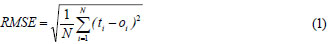
where:

N is the number of data sets.

t_i is the target value for the i^th set.

o_i is the output of the i^th set which is produced by the ANN

The RMSE is then propagated backwards to the input layer and the connection weights between the layers are readjusted. After the weights have been adjusted and the hidden layer nodes have generated an output result, the error value is re-determined. If the error value was not reached, which is usually defined by a particular iteration number, the error will then again be propagated backwards to the input layer. This procedure continues until the model has finally reached the predetermined tolerance limit. To decrease the initial learning rates, a learning coefficient ratio is used. The learning coefficient is reduced from the initial learning coefficient by an amount corresponding to the learning coefficient ratio until training time. In this respect, even if initially high learning rates are selected, such as 0.3 for the hidden layer and 0.15 for the output layer, and the momentum coefficient is selected as 0.4, the training of the network can be accomplished, in this example, with a 0.00001 learning rate and a 0.00001 momentum coefficient after 50 000 iterations.

The overall data set was divided into 2 subsets for each analysis: training and testing. We used 75% of the data for training and 25% of the data for testing. The training and testing data sets were selected randomly. Furthermore, the minimum and maximum values for the data range for each data set were considered very carefully. Since the ANN predictions are valid within the trained and tested data range, as is the case for any model, the data range must be selected very carefully. This problem was neglected by some of the studies reported in the literature.

Parameter descriptions

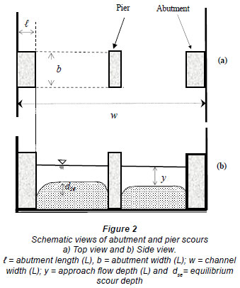
Laboratory data for the equilibrium local scour depth around abutments, for the clear-water condition, obtained by 7 investigators, were used for this study. Scour is a time-dependent phenomenon. However, under constant flow conditions stable position is reached after a certain time period, after which scour will not increase further. The depth of scour at this stage is called either the equilibrium scour depth or maximum scour depth. The depth of maximum scour is a design parameter. A schematic description of a bridge foundation composed of piers and abutments is shown in Fig. 2. Since the data pertain to local scour, the shape of the abutment is important as a physical quantity. The abutment shape for all of the experimental data analysed in the present study was a vertical wall, as seen in Fig. 2.

 

 

For below or near clear-water approach flow conditions, the equilibrium local scour depth, d,_se at an abutment is a function of fluid, flow, sediment, geometry of both channel and structure, and time, as given in Eq. (2).

where:

u = mean approach flow velocity (LT^-1)

y = approach flow depth (L)

g = gravitational acceleration (LT^-2)

r = density of the fluid (ML^-3)

m = dynamic viscosity of fluid (ML^-1T^-1)

ρ_s = density of the sediment (ML^-3)

d₅₀ = median particle grain size (L)

σ_g = (d₈₄/dj₁₆)^0.5, the geometric standard deviation of sediment size distribution (d₈₄ = sediment size for which 84% of the sediment is finer, d,₁₆ = sediment size for which 16% of the sediment is finer)

= abutment length (L)

b = abutment width (L)

w = channel width (L)

S_o = slope of the channel (L/L)

t = scouring time (T)

The Buckingham π theorem will reduce Eq. (2) to 11 dimensionless variables as follows:

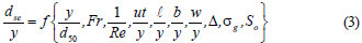
Fr is the Froude number and Re is the Reynolds number, and Δ is the dimensionless density parameter which is described as:

The dimensionless parameters are necessary while applying regression analysis by reducing the number of parameters. However in ANN modelling we have the freedom to select the number of nodes at the input layers, therefore the use of raw data instead of dimensionless parameters will be a better choice. Evidence from the literature also shows that ANN models are not performing well with dimensionless parameters. Kambeker and Deo (2003) used raw data as input but predicted a dimensionless form of the scour depth. Although they used both forward feed and recurrent neural network models and 2 learning algorithms; back-propagation and cascade correlation, the results only changed slightly. Bateni et al. (2007b) concluded that use of constitutive raw parameters in place of their group yields better results because of the increased flexibility in fitting which is achieved. In the study of Bateni et al. (2007a), a sensitivity analysis of the dimensionless parameter was carried out, which showed that y/b_pier was the most effective and Reynolds number, Re, was the least effective parameter. In the same study, sensitivity analysis with raw data shows that the pier diameter is the most important parameter. However, the pier diameter is included in both dimensionless (normalised) parameters of the most effective parameter, y/b_pier, and the least effective parameter, Re. It can thus be concluded that dimensionless variables are not useful in ANN models. In Liriano and Day's study (2001) the dimensionless group gives a slightly better prediction of scour at the culvert outlets. This is the only exception which was found in the literature. Therefore, we choose the raw data for the following analysis.

 

Can data collected by different researchers at different times be gathered in 1 set?

The sample size of the total measured data of 7 researchers was 85; Table 1 shows the characteristics of these 7 data groups (which were sourced from Ballio (2004) and were used in studies published in: Ballio and Orsi, 2000; Tey, 1984; Dongol, 1994; Ladage, 1998; Rajaratnam and Nwachukwu, 1983; Cunha, 1975; Oliveto and Hager, 2002). Each data group in Table 1 is named using 'D' followed by a number. In this table, only the maximum and minimum values of the measured quantities are presented due to space limitations.

Thus, at the first stage of the study in ANN modelling, flow depth, y, abutment length, I, abutment width, b, median particle grain size, d50, and mean approach flow velocity, u, were input variables and the equilibrium scour depth, d_se, was the target output. These variables are most common variables observed in the laboratory and field studies.

After using randomly-selected data sets for training (70) and testing (15), the root mean square error (RMSE) and the correlation coefficient (R²) of the test case were found to be 0.2601 and 0.43, respectively. The correlation coefficient of 0.43 and RMSE value of 0.261 used for quantitative comparisons are not high enough to establish an accurate and reliable model. At this stage, it can be concluded that this ANN model failed to obtain good results for this data set, suggesting that a new model should be found which yields reasonable results from available data set. However, instead of finding a new model, the same ANN model was used to scrutinise the data set in order to investigate the following question: Can data collected by different researchers at different times be gathered in 1 data set?

To find the answer to the above question, Total Data (TD) was examined for each researcher. Thus, each data subset was extracted from Total Data one by one and an ANN model was constructed for each case. In Table 2, these results are presented with the result of TD including 5 input variables (TD5).

 

 

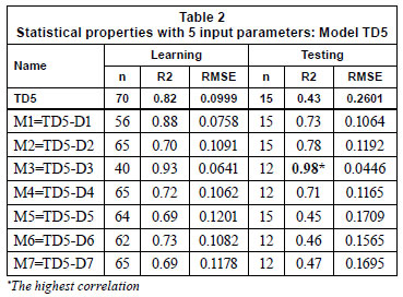
Investigating the statistical output (given in Table 2), it can be seen that the correlation coefficients are increased and the highest correlation value of 0.98 is obtained when D3 is subtracted from the total data. Therefore, M₃ can be selected as a design model. Then each subset was taken as test data and the performance of the selected model, M₃, was evaluated. Table 3 shows the results of these model runs.

 

 

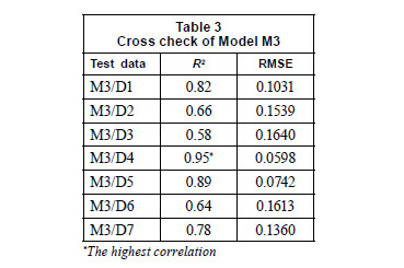
According to the results presented in Table 3, it can be concluded that our experimental data sets should not be gathered in 1 set, since the data set of D3 is not consistent with the others.

 

Can we determine any unquantified effects such as differences in heterogeneity of data, laboratory conditions and measurement devices?

The purpose of this stage was to determine some unquantified effects such as data difference, laboratory conditions and measurement devices on examined data sets. As can be seen in Table 3, while the lowest correlation is obtained with M₃/D3, the highest correlation is obtained with M₃/D4. Thus, D3 data produce a poorer estimate compared to the rest of the data sets.

This may be due to the fact that D3 data are not consistent with the other data subsets. To investigate further, it was decided that the number of input data would be increased by including geometric standard deviation of sediment size distribution, a , and dimensionless sediment density parameter, Δ.

A question arises at this stage about the inclusion of critical mean velocity, u_c, since in conventional regression analysis the use of critical velocity is very common. Also, in the literature, critical velocity, u_c is included in the input list for an ANN model (Muzammil, 2008). However, u_c should be ignored because the critical mean velocity for entraining bed sediment can be estimated from y and d₅₀ (Melville and Coleman, 2000) in order to obtain an independent input set. There are a few empirical equations proposed for the phenomena including critical velocity. The critical velocity has importance when observing or analysing time-dependent scour. Therefore, both the critical velocity and equilibrium scour time were accounted for in the study of Bateni et al. (2007b); in addition it was shown that critical velocity is the least effective parameter.

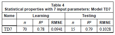
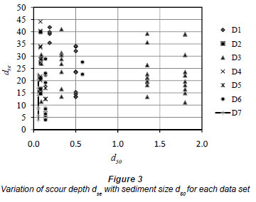
Table 4 summarises the results for the model with 7 input parameters. The correlation coefficient is raised to a value of 0.79. Therefore, it can be said that both the sediment size and its uniformity are effective parameters for predicting abutment scour. In order to emphasize this conclusion, subset D3 can be inspected to find out whether it includes coarse sediment or not. Figure 3 shows d_se as a function of d₅₀ for each data subset. It is seen that D3 contains coarse sediment (d₅₀>1 mm), meaning that D3 subset is not compatible with the other subsets due to the range of sediment diameters. Therefore, instead of excluding the whole D3 dataset, only the coarse sediment data from D3 were excluded from the total data.

 

 

 

 

The correlation coefficient and RMSE values for the new model excluding the coarse sediment data of D3 were computed as 0.77 and 0.11178, respectively (see Table 5). The new correlation coefficient is higher than TD5 (0.43) but lower than TD7 (0.79) model. To examine this result in detail, geometric standard deviation, σ_g, of particle size distribution, which is a measure of uniformity of the bed sediments, was investigated. Thus, it is considered whether the data subsets contain uniform or non-uniform sediments. This is important because non-uniform sediments (σ_g >1.4) consistently produce lower scour depths than uniform sediments. Variations of scour depths dse with sediment gradation σ_g for each data set are shown in Fig. 4.

 

 

 

 

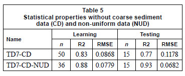
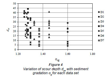
According to Fig. 4, some D3 and D6 data points are greater than 1.4. Therefore, these data were also excluded from the total data and the analysis was repeated without coarse and non-uniform sediment data. The correlation coefficient and RMSE values were computed and are given in Table 5. The correlation coefficient increased to a value of 0.93.

This exercise showed that misinterpretation can easily occur, regardless of the accurateness of the model, unless the number of data points and the number of parameters is large enough to address the problem.

 

Sensitivity analysis

In the last part of this study, a sensitivity analysis was carried out to identify the dominant parameters influencing the problem. Table 6 shows the result of the sensitivity analysis for 7 parameters with the reduced data set, after excluding the experiments with the coarse and non-uniform sediments. In the process of the sensitivity analysis, the parameters were excluded one by one from the list of input variables. Then, the parameter with the least relative importance compared to all of the other parameters is extracted from the model construction, based on the highest correlation coefficient. This procedure is repeated for all parameters one by one. In the first stage, the least effective parameter was determined to be abutment width, b, since the highest correlation is obtained when b is excluded from the input list. This conclusion has been supported by experimental research reported by Kayatiirk (2005). Therefore, in the second stage, b was omitted, and the analysis repeated for the rest of the variables. In Table 6, the results are given for different hidden nodes, and it can be seen that increasing the number of hidden nodes is not necessary for improving the results. In summary, the parameters can be listed from the least effective to the most effective as follows: b, d50, Δ,σ_g , y, and u.

 

Discussion

In general, when constructing an ANN model, parameters are selected according to available empirical equations in the literature. Some researchers have tried to compare their results with the available equations based on the results of regression models. For example, Choi and Cheong (2006) and Firat and Gungor (2009) compared results of ANN models developed to predict bridge pier scour with some of the available empirical calculations. Choi and Cheong (2006) used the equations of Laursen and Toch (1956), Neill (1973), Jain and Fisher (1979), CSU (Richardson and Davis 1995) and Melville (1997). The results showed that CSU gave the minimum error. Jain and Fisher (1979) and Melville (1997) over-predicted the scour depth. Among 5 formulas, only CSU encompasses b_pier, y, u, d₅₀ , and σ_g , whereas Melville's formula contains u_c instead of u and Jain and Fisher include u and u_c , together. Furthermore, Laursen and Toch (1956) and Neill's (1973) formulas consist of only 2 parameters, b_pier and y. These results showed that the consistency of the number of parameters between different models is quite important in order to establish model superiority. Firat and Gungor (2009) compared experimental data of several researchers with 5 empirical equations reported in the literature. In their study no information is given on the selection of the 5 equations. Equations based on regression analysis of experimental data always have limitations due to the range of parameters. If the equations are the result of linear regression, it is obvious that a model which is able to predict non-linear relationships can give better results. However, the knowledge which can be gained from such laboratory studies should not be underestimated.

Therefore, ANN models or more advanced models can be powerful tools if the data base is large enough to cover as many different conditions as possible. It is widely accepted that ANN models are universal approximators. However, according to Hornik et al. (1989), an ANN can act as a universal function approximator if a sufficiently long training time and sufficiently large number of hidden layers with a sufficiently large number of neurons in each of the hidden layers are given. Moreover, ANN models are data intensive (ASCE, 2000). If the number of data is limited, extra effort should be invested in selecting the model parameters. In addition, the homogeneity of data has great importance.

 

Summary and conclusions

An artificial neural network model is used as a tool to analyse the experimental data for equilibrium local scour depth around bridge abutments. The ability of ANN models in establishing relations with different data groups is investigated and the reasons for the effectiveness of ANN models for these data sets were examined. This study exposes that researchers need to be careful when gathering different experimental or field data sets together before constructing an ANN model since the model is data driven.

For the first part of the study, a general ANN model with 5 input parameters was constructed with the total data (85) classified as training (70) and testing (15). A data elimination process was then performed by subtracting each data subset from the total data set, one by one. This procedure showed whether each subset had similar characteristics or not.

For the second part of the study, 7 input parameters were used and each data subset was analysed in detail. The detailed analysis of each data subset indicated the importance of parameter number and data homogeneity. The results confirm that ANN models can successfully be used to trace the compatibility of the experimental data collected from different studies.

In the last part of the study, sensitivity analysis was carried out to discover the dominant parameters of the problem. Sensitivity analysis demonstrated that flow mean velocity, u, is the most effective, and abutment width, b, is the least effective parameter for determining equilibrium scour depth, d_se.

In conclusion, the findings of the present study, along with other published studies, show that with available algorithms and data we are actually still far from reaching a universal conclusion for scour depth calculations. It is suggested that the community of hydraulic engineers should collaborate in order to establish a data bank for this problem.

 

Acknowledgements

The authors are indebted to Assoc. Prof. Francesco Ballio for supplying the experimental data. Funding for this project was partially provided by TUBITAK (Turkish National Science Foundation) under Grant ICTAG 102I068.

 

References

ADELI H and YEH C (1989) Perceptron learning in engineering design. Microcomput. Civ. Eng. 4 247-256.        [ Links ]

ASCE (AMERICAN SOCIETY OF CIVIL ENGINEERS) (2000) Task Committee on Application of Artificial Neural Networks in Hydrology, Artificial Neural Networks in Hydrology II: Hydrology Application. J. Hydrol. Eng. 5 (2) 124-137.        [ Links ]

AZAMATHULLA HM, AB GHANI A, ZAKARIA NA and GUVEN A (2010) Genetic programming to predict bridge pier scour. ASCE J. Hydraul. Eng. 136(3)165-169.        [ Links ]

BALLIO F (2004) Assoc. Prof. Francesco Ballio, personal communication, 24 June 2004, Politecnico di Milano, Piazza Leonardo da Vinci 32, 20133, Milano, Italy.        [ Links ]

BALLIO F and ORSI E (2000) Time evaluation of scour around bridge abutments. Water Eng. Res. 2 243-259.        [ Links ]

BARBHUIYA AK and DEY S (2004) Local scour at abutments: A review. Sadhan 29(5)449-476.        [ Links ]

BATENI SM, BORGHEI SM and JENG DS (2007a) Neural network and neuro-fuzzy assessments for scour depth around bridge piers. Eng. Appl. Artif. Intell. 20 401-414.        [ Links ]

BATENI SM, JENG DS and MELVILLE BW (2007b) Bayesian neural networks for prediction of equilibrium and time-dependent scour depth around bridge piers. Adv. Eng. Software 38 102-111.        [ Links ]

BEGUM SA, KASHIM A and BARBHUIYA AK (2011) Radial basis function to predict scour depth around bridge abutment. URL: http://ieeexplore.ieee.org/stamp/stamp.jsp?arnumber=05751387 (Accessed May 2011).        [ Links ]

BRICE JC and BLODGETT JC (1978) Countermeasure for Hydraulic Problems and Bridges, Volumes 1 and 2. Federal Highway Administration, U.S. Dept. of Transportation, Washington, D.C.        [ Links ]

CHOI SU and CHEONG S (2006) Prediction of local scour around bridge piers using artificial neural networks. J. Am. Water Resour. Assoc. 42(2)487-494.        [ Links ]

CUNHA LV (1975) Time evolution of local scour. Proc. 16th Conf. Int. Assoc. Hydraulic Research (Delft: IAHR). 285-299.        [ Links ]

DONGOL DMS (1994) Local Scour at Bridge Abutments. Report No. 544, School of Engineering, University of Auckland, Auckland, New Zealand.        [ Links ]

ETTAMA R, NAKATO T and MUSTE M (2003) An overview of scour types and scour estimation difficulties faced bridge abutments. Proc. Mid-Continent Transportation Research Symposium, 21-22 August 2003, Iowa.        [ Links ]

FHWA (FEDERAL HIGHWAY ADMINISTRATION, UNITED STATES) (2001) Evaluating scour at bridges. Publication No. FHWA NHI 01-001, HEC No. 18. USA National Highway Institute.        [ Links ]

FIRAT M and GUNGOR M (2009) Generalized regression neural networks and feed forward neural networks for prediction of scour depth around bridge piers. Adv. Eng. Software 40 731-737.        [ Links ]

GRAF WH (2001) Fluvial Hydraulics: Flow and Transport Processes in Channels of Simple Geometry. In collaboration with MS Altinakar. John Wiley and Sons, London.        [ Links ]

HORNIK K, STINCHCOMBE M and WHITE H (1989) Multilayer neural networks are universal approximators. Neural Networks 2 256-366.        [ Links ]

JAIN SC and FISHER EE (1979) Scour around bridge piers at high Froude number. Report No. F.H.W.A.R.D. 79-104. Federal Highway Administration, Washington DC.        [ Links ]

KAMBEKAR AR and DEO MC (2003) Estimation of pile group scour using neural networks. Appl. Ocean Res. 25 225-234.        [ Links ]

KANDASAMY JK and MELVILLE BW (1998) Maximum local scour depth at bridge piers and abutments. J. Hydraul. Eng. 36(2)183-198.        [ Links ]

KAYA A (2010) Artificial neural network study of observed pattern of scour depth around bridge piers. Comput. Geotechnics 37 423-418.        [ Links ]

KAYATURK (KUMCU) SY (2005) Scour and Scour Protection at Bridge Abutments. Ph.D. Thesis, Middle East Technical University, Turkey.        [ Links ]

KOTHYARI UC and RANGA RAJU KG (2001) Scour around Spur Dikes and Bridge Abutments. J. Hydraul. Res. 39(4)367-374.        [ Links ]

LADAGE F (1998) Temporal development of local scour at bridge abutments. Internal Report, Department of Civil and Resource Engineering, University of Auckland, Auckland, New Zealand. 39 pp.        [ Links ]

LAURSEN EM and TOCH A (1956) Scour around Bridge Piers and Abutments. Bulletin No. 4., Iowa Road Research Board.        [ Links ]

LAURSEN EM (1962) Scour at bridge crossings. Trans. ASCE127 (1) 166-209.        [ Links ]

LEE TL, JENG DS, ZHANG DS and HONG JH (2007) Neural network modeling for estimation of scour depth around bridge piers. Hydrodyn. 19(3)378-386.        [ Links ]

LIRIANO SL and DAY RA (2001) Prediction of scour depth at culvert outlets using neural networks. J. Hydroinf. 3(4)231-238.        [ Links ]

MACKY GH (1990) Survey of Roading Expenditure due to Scour. C.R. 90.09. Department of Scientific and Industrial Research (DSIR), Hydrology Centre, Christchurch, New Zealand.        [ Links ]

MELVILLE BW (1997) Pier and abutment scour: Integrated approach. J. Hydraul. Eng. 123(2)125-136.        [ Links ]

MELVILLE BW and COLEMAN SE (2000) Bridge Scour. Water Resources Publications, Colorado.        [ Links ]

MUZZAMMIL M (2008) Application of neural networks to scour depth prediction at the bridge abutments. Eng. Appl. Comp. Fluid Mech. 2(1)30-40.        [ Links ]

NEILL CR (1973) Guide to Bridge Hydraulics. Roads and Transportation Association of Canada. University of Toronto Press. 191 pp.        [ Links ]

NEURALWARE INC. (2002) Neural Works Professional II Plus. NeuralWare Inc., Carnegie (USA).        [ Links ]

OLIVETO G and HAGER WH (2002) Temporal evolution of clear-water pier and abutment scour. J. Hydraul. Eng. 128 811-820.        [ Links ]

PAL M, SINGH NK and TIWARI NK (2011) Support vector regression based modeling of pier scour using field data. Eng. Appl. Artif. Intell. 24 911-916.        [ Links ]

RAHMAN HS, ALIREZA K and REZA G (2010) Application of artificial neural network, kriging and inverse distance weighting models for estimation of scour depth around pier and bed sill. J. Software Eng. Appl. 3 944-964.        [ Links ]

RAJARATNAM N and NWACHUKWU BA (1983) Flow near groinlike structures. J. Hydraul. Eng. 109 463-480.        [ Links ]

RICHARDSON JE and DAVIS SR (1995) Evaluating Scour at Bridges. Report No. FHWA-IP-90-017, Hydraulic Engineering Circular No. 18 (HEC-18) (3^{r d} Edn.). Office of Technology Applications, HTA-22, Federal Highway Administration, U.S. Department of Transportation, Washington D.C.        [ Links ]

RUMELHART DE, HINTON GE and WILLIAMS RJ (1986) Learning internal representation by error back propagation. In: Rumelhart DE and McClelland JL (eds.) Parallel Distributed Processing. MIT Press, Cambridge MA. 318-362.        [ Links ]

SARLAK N, TIGREK S and KAYATURK Y (2006) Prediction of the scour depth around bridge abutments by using ANN. Proc. 7th Int. Conf. on Hydroinformatics, HIC, 4-8 September 2006, Nice, France.        [ Links ]

SHIRHOLE AM and HOLT RC (1991) Planning for a Comprehensive Bridge Safety Program. Transportation Research Record 1290, Vol. 1. Transportation Research Board, National Research Council, Washington DC. 39-50.        [ Links ]

STURM TW and SADIQ A (1996) Clear-water scour around bridge abutments under backwater conditions. Transportation Research Record 1523, Transportation Research Board, National Research Council, Washington, DC. 196-202.        [ Links ]

SUTHERLAND AJ (1986) Reports on Bridge Failure. R.R.U. Occasional Paper, National Roads Board, Wellington, New Zealand.        [ Links ]

TEY CB (1984) Local scour at bridge abutments. Report No. 329, School of Engineering, University of Auckland, Auckland, New Zealand.        [ Links ]

YANMAZ AM (2002) Kopru Hidroligi. METU Press, Ankara.        [ Links ]

ZOUNEMAT-KERMANI M, BEHESHTI AA, BEHZAD AA and SABBAGH-YAZDI SR (2009) Estimation of current-induced scour depth around pile groups using neural network and adaptive neurofuzzy inference system. Appl. Soft Comput. 9 746-755.        [ Links ]

 

 

Received 17August 2010; accepted in revised form 5 September 2011.

 

 

* To whom all correspondence should be addressed. (90)-342-3172421; fax: (90)-342-3172410; e-mail: sarlak@gantep.edu.tr