Input variable selection for interpolating high-resolution climate surfaces for the Western Cape

 

 

Adriaan van Niekerk^I,*; Sarah Joan Joubert^II

^ICentre for Geographical Analysis, Stellenbosch University, Private Bag X1, Matieland 7602, South Africa
^IIGeography and Environmental Studies, Stellenbosch University, Private Bag X1, Matieland 7602, South Africa

 

 

---

ABSTRACT

Accurate climate surfaces are vital for applications relating to groundwater recharge modelling, evapotranspiration estimation, sediment yield, stream flow prediction and flood risk mapping. Interpolated climate surface accuracy is determined by the interpolation algorithm employed, the resolution of the generated surfaces, and the quality and density of the input data used. Although the primary input data of climate interpolations are usually meteorological data, other related (independent) variables are frequently incorporated in the interpolation process. One such variable is elevation, which is known to have a strong influence on climate. This research investigates the potential of 4 additional variables for inclusion in the interpolation process. Three of the variables, namely, slope gradient, slope aspect and hillshade, are related to topography, while the fourth is related to large water bodies (i.e. distance to oceans). Correlation analyses were used to determine the suitability of each of the 4 variables for interpolating climate surfaces in the Western Cape Province, South Africa. Although moderate correlations were identified between climate records and distance to oceans, no significant correlation was found for slope gradient, slope aspect and most variations of hillshade. However, a moderate correlation was identified between rainfall records and hillshade with a 180º azimuth. This variable was consequently used in various combinations with distance to oceans and elevation to generate 8 sets of high-resolution (i.e. 3 arc second) climate surfaces of the Western Cape. According to an accuracy assessment of the resulting surfaces, distance to oceans reduced the mean error of monthly mean maximum daily temperature interpolations by 27%. Distance to oceans also improved the accuracy of monthly mean minimum daily temperature interpolations for October through April. Although hillshade (180º azimuth) did not improve accuracies for temperature interpolations, it did improve the accuracy of monthly rainfall surfaces for 4 months of the year. The combinations of input variables that produced the lowest monthly mean errors were used to generate a new set of surfaces using all available meteorological data. A pair-wise comparison of the new interpolated surfaces with existing climate surfaces revealed that the surfaces created using our methodology are, in general, more accurate than any existing interpolations.

Keywords: climate, surface, interpolation, rainfall, temperature

---

 

 

Introduction

Accurate climate data are vital for hydrological applications such as groundwater recharge modelling (Archer et al., 2009; Wassenaar et al., 2009), evapotranspiration estimation (Siebert and Döll; 2010, Zhu et al.), sediment yield (Faran Ali and de Boer, 2008), stream flow prediction (Besaw et al., 2010) and flood risk mapping (Bradshaw et al., 2007). Spatially interpolated climate data, or climate surfaces, are also important in agricultural applications, particularly those related to land suitability analysis (Fourie, 2006; Van Niekerk, 2008), terroir studies (Carey, 2005) and crop-water management (Huang and Li, 2010). Unfortunately, the resolution and accuracy of existing spatially interpolated climate data are often not sufficient for applications on regional and local scales. This is true for the Western Cape Province of South Africa, where the increasing use of geographic information systems (GIS) to support environmental and water management decisions has led to a growing need for high-resolution climate surfaces. A requirement analysis (Van Niekerk, 2008) revealed that such data should be suitable for use at large mapping scales (i.e. 1:50 000 or larger) and be accurate enough to support decisions at a local level.

Contrary to some studies (e.g. Hutchinson et al. (1984); Sharples et al. (2005)) that have shown that the accuracies of interpolated climate surfaces, particularly those related to rainfall, do not necessarily improve with fine spatial resolutions, Hijmans et al. (2005) suggests that climate surface accuracy strongly relates to surface resolution as climate variation is often lost at lower spatial resolutions. Interpolated surfaces with high resolutions are therefore more likely to accurately represent climate variation at large mapping scales.

The accuracy of climate surfaces is also directly influenced by the quality and density of input data and the robustness of the interpolation algorithm. Although the primary input data of climate interpolations are usually weather station data, other related (independent) variables are frequently incorporated in the interpolation process. One such variable is elevation, which is known to have a strong influence on climate. Slope gradient and aspect are frequently used as additional variables to permit the incorporation of topographical effects on temperature and rainfall, while distance to large water bodies are often used to simulate the effect that oceans and lakes have on climate (Hutchinson, 1998).

This research investigates the potential effects of 4 additional variables on climate surface accuracy when using the well-documented (Hutchinson, 1989; Hutchinson, 1998; Hutchinson, 1998; Hutchinson, 2011; Hutchinson et al., 1996) and popular (Chapman, 2000; Funk and Richardson, 2002; Hijmans et al., 2005, Jakob et al., 2005; Jeffrey et al., 2001; McKenney, 2000; Price et al., 2000; Zuo et al., 1996) thin-plate smoothing spline interpolation algorithm of the ANUSPLIN software. Three of the variables that were investigated, namely, slope gradient, slope aspect and hillshade, are related to topography, while the fourth is related to large water bodies (i.e. distance to oceans). Hillshade was incorporated as an additional variable as it combines slope gradient and aspect and was expected to better emulate the effect of weather patterns in mountainous regions (e.g. rain shadows). Correlation analyses were used to determine the suitability of each of the 4 variables in the creation of climate surfaces for the Western Cape. The variables deemed to have a direct influence on the study area's climate were used in various combinations to generate 8 sets of high-resolution (i.e. 3 arc second) climate surfaces. The accuracy of the resulting surfaces was assessed using reference data to determine the best combination of input variables.

 

Study area

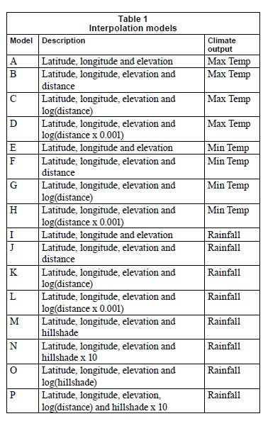
The Western Cape Province (Fig. 1) is situated in south-western South Africa and covers an area of 129 370 km² (Winter, 2002). The province is bordered seaward by the Indian Ocean in the south and the Atlantic Ocean in the west, while the northern and eastern parts of the province are bounded by other South African provinces.

The Western Cape's topography is complex, ranging from coastal plains to complex mountain ranges and valleys. The topography is dominated by the Cape Fold Belt, forming L-shaped mountain ranges oriented in a north to south and east to west direction. Three distinct climatic regions, namely, the Mediterranean, South Coast, and Karoo regions, are recognisable (Fig. 1). The Mediterranean region, located in the western and south-western parts of the Western Cape, receives most of its rainfall during the winter (May to August) (Fig. 2). This is mainly due to the influence of the cold Benguela current of the Atlantic Ocean and the northward displacement of high-pressure systems during winter, allowing westerly winds to introduce cold polar air to the region. Winters are mild to cool, while summers are warm to hot. Although most of the Mediterranean region's rainfall is received as prefrontal rain and postfrontal showers, rainfall variability is high due to heavy orographic rainfalls (South African Weather Bureau, 1996).

 

 

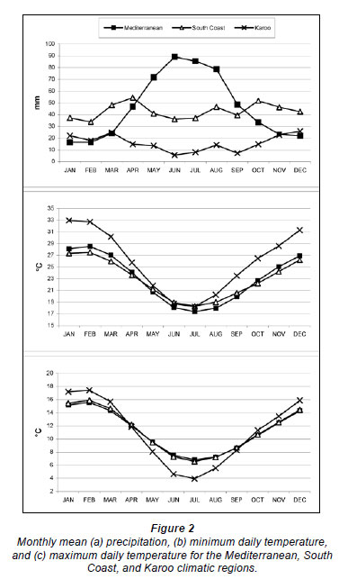
In contrast, the South Coast region - extending eastward from Cape Agulhas - experiences rainfall throughout the year. Rainfall is principally a result of the movement of moist, warm air from the Indian Ocean and orographic influences. As a result, the southern mountain slopes generally receive more rainfall than the northern slopes. Although the weather is warm during the summer and mild during winter, a marked decrease in temperature is experienced with an increase in altitude. The effect of the Indian Ocean does not extend farther than the mountain ranges which form a natural divide between the South Coast and Karoo climate regions. The Karoo region is confined to the inland plateau of South Africa and receives most of its rainfall during late summer, mainly in the form of thundershowers. Rainfall in this semi-arid region is low and unreliable, while temperatures vary considerably from winter to summer (South African Weather Bureau, 1996).

 

Climate surface interpolation

Because an area's climate is an aggregate of its weather conditions over time (Lutgens and Tarbuck, 1998), reliable climate data can only be obtained through statistical analyses of weather observations (Houghton et al., 2001). Unfortunately, weather stations are often sparsely distributed, especially in mountainous regions or areas with low population densities, resulting in vast regions being insufficiently represented by weather stations. Interpolation methods are frequently employed to estimate climate data for areas that are near weather stations. The accuracy of such estimations is a function of input data accuracy, spatial variability and the interpolation method employed (Hartkamp et al., 1999).

The quality of weather data, which are the primary source of input to the interpolation process, will greatly influence the accuracy of any interpolation. Generally, higher densities of weather stations will provide better results. Apart from density considerations, weather data should also represent as long a period as possible, typically more than 30 years, to reduce the effect of temporal climate variations.

The type of algorithm used in climate interpolations is especially important when data are used from sparsely-spread weather stations. Several interpolation methods, ranging from deterministic (e.g. Thiessen polygons and inverse distance weighting) to stochastic (e.g. polynomial regression, trend surfaces and kriging) have been used to generate climate rasters. Thin plate splining is, however, recommended in data sparse areas (Price et al., 2000). Like Kriging, many splining algorithms also provide predictions of uncertainty (or error surfaces) that can be used to describe the spatial quality of the results and incorporate independent variables (or covariates), such as elevation and distance to oceans, to improve the accuracies of the interpolated surfaces. In addition, splining is computationally simplistic, which is particularly important when rasters are created for large areas and/or have high resolutions (Hijmans et al., 2005, Price et al., 2000). These attributes of splining algorithms are likely to be the reason why they are often used in interpolation comparative studies and climate surface creation analyses (Jarvis and Stuart, 2001; Vicente-Serrano et al., 2003).

The spline method can be conceptualised as fitting a rubber-sheeted surface through the known points using a mathematical function. In fitting surfaces to data points, thin-plate smoothing splines determine an optimal trade-off between accuracy of fit and surface smoothness by minimising the generalised cross-validation (GCV). The GCV value is an estimate of the interpolation error obtained by removing each data point in turn and fitting a spline surface to the remaining data to see how well each omitted point can be predicted (Hutchinson et al., 1996).

ANUSPLIN, developed by the Australian National University (Hutchinson, 2011), is possibly the most popular thin-plate smoothing spline interpolation algorithm available. ANUSPLIN has been applied at regional level in New Zeeland (Tait et al., 2006), Canada (Price et al., 2000), Madagascar (Chapman, 2000), China, Thailand, Vietnam, Laos, Cambodia and the Malay Peninsula (Zuo et al., 1996), and Guyana (Funk and Richardson, 2002). It has also been used to develop continental-scale climate surfaces for Australia (Jakob et al., 2005; Jeffrey et al., 2001), Africa (Hutchinson et al., 1996) and North America (McKenney, 2000), and has more recently been used for the WorldClim international data set (Hijmans et al., 2005).

 

Methods

This research involved statistical analyses of climate-related data and the interpolation of climate surfaces for the Western Cape. The following sections overview the methods employed.

 

Climate data collection and preparation

Long-term rainfall and temperature data were collected for weather stations in and around the Western Cape (see Fig. 1). The main sources of weather station data were the South African Weather Services (SAWS) and the Agriculture Research Council (ARC). Stations with collecting periods shorter than 10 years were not considered, resulting in a data set for 125 stations and an average collection period of 30 years. Although the overall density of weather stations is relatively high (1 station for every 2 285 km²), the density is notably lower in the northern, less-populated parts of the province. Consequently, all stations situated up to 100 km outside the Western Cape were included to enhance the accuracy of the spline function calculations in the northern parts of the province.

Weather station data are treated by most climate surface interpolation algorithms as being dependent on latitude, longitude and elevation (Barringer and Lilburne, 2000). Elevation is usually incorporated in the interpolation algorithm as a digital elevation model (DEM). For this purpose, the 3-arc-second (approximately 90 m) resolution Shuttle Radar Topography Mission (STRM) DEM (United States Geological Survey, 2006) was used, owing to its high resolution and high degree of accuracy (Rodriguez et al., 2005).

In addition to elevation, other topographic variables and factors, such as ocean proximity, can also be used as independent variables or covariates in the interpolation process (Price et al., 2004). ArcGIS was used to derive slope gradient, slope aspect and hillshade from the STRM DEM. The algorithm used to compute a hillshade value for each cell is R_f = cos(A_f - A_s)sin(H_f)cos(H)+cos(H_f)sin(H_s) with R_f the relative radiance of a raster cell, A_f the aspect of the cell, A_s the sun's azimuth, H_f the cell's slope and H_s the sun's altitude. R_f ranges in value from 0 to 1 and is multiplied by a constant 255 to obtain the illumination value (Chang, 2010). Various hillshades with different azimuths and sun altitude values were generated using this method.

ArcGIS was also used to calculate distances to the nearest ocean. To do so, coastline data were obtained from the Chief Directorate: National GeoSpatial Information of South Africa. All the input data sets were generated at a resolution of 3-arc-seconds to match the resolution of the input DEM. Although lower resolutions were considered to reduce computational processing requirements, it was decided to produce climate surfaces at the highest possible resolution to eliminate the effects that resampling might have on the output accuracy. It is, however, unlikely that the resulting surfaces will be representative of 3-arc-second weather patterns as other factors, such as land cover, albedo and wind, will also influence local scale climate variability.

 

Input variable elimination using correlation analyses

Standard Pearson's product-moment correlation coefficients were calculated for each combination of dependent (mean daily maximum temperature, mean daily minimum temperature, and mean rainfall) and candidate independent (slope gradient, slope aspect, distance to oceans, and hillshade, respectively) variables on a monthly basis. This process enabled the identification and elimination of candidate input variables that have no significant relationship with meteorological records. Only distance to oceans and one variation of hillshade (with 180º azimuth and 45º altitude) showed significant correlations with the weather station data. The other candidate variables (slope gradient, slope aspect and all other variations of hillshade) were consequently eliminated from further analysis using this methodology.

 

Climate surface generation

Only those variables for which a significant correlation with climate records was found were considered for generating climate surfaces. Input variables were incorporated in ANUSPLIN as dependent variables, independent variables or covariates. Latitude and longitude were defined as independent variables for all interpolations, while elevation was interpreted as a covariate instead of independent variable when additional variables (e.g. distance to oceans) were considered in the interpolation (Hutchinson, 2011). Additional variables were also designated as covariates in such cases. Some input variables required scaling prior to interpolation. Through experimentation during preliminary analyses it was found that Hutchinson's (1998) square-root transformation of rainfall data produced the best results. A similar approach was taken to find suitable transformations for additional variables. These included square-root and logarithmic transformations as well as scaling (multiplication) by 0.001, 0.01. 0.1, 10, 100 and 1 000.

With the purpose of identifying suitable transformations and units for the additional variables, various possibilities for the distance to ocean and topography (aspect and slope) variables were investigated. In order to test the accuracy of the range of options, ANUSPLIN provides a series of statistical outputs which can be used for performance analysis (Hutchinson, 1998a; b; Price et al., 2000).

The interpolation of the climate surfaces was carried out for the entire study area. Splining is a deterministic interpolator with a stochastic component, which means that only a specified number of neighbouring points are used to determine an unknown value (Burrough and McDonnel, 1998). It is consequently unlikely that the mesoscale processes in one climate region will influence the interpolated values of another.

The SPLINA module of ANUSPLIN was used as the interpolation algorithm. The configuration of SPLINA was guided by Hutchinson's (1998) prescriptions. Second-order spline functions were used for trivariate models (i.e. those using only longitude, latitude and elevation as input) and when a fourth variable was incorporated as a covariate. Third-order spline functions were used when a fourth variable was included as independent variable or when a fifth variable was used.

 

Accuracy assessments

To investigate the effect of the candidate variables on climate surface interpolation accuracy, all permutations of additional variables were considered. Sets of 12 interpolations each (one for each month) were generated from a stratified 80% random sample of the available weather station data. The sample was stratified based on the 3 weather station density zones shown in Fig. 1. Data from the remaining (20%) weather stations were withheld from the interpolation process and used to calculate mean error. Error margins of 0.5ºC for temperature and 10-30% for rainfall, as suggested by Hutchinson et al. (1996), were used as a guideline for accuracy.

The accuracy assessment based on the 20% sample was supplemented by the interpolation software's own statistical outputs for performance analysis (Hutchinson, 1998; Hutchinson, 1998; Price et al., 2000). These measures included the root of the generalised cross-validation (RTGCV), the root of the mean square residual (RTMSR) and the root of the mean square error (RTMSE). The RTGCV values are conservative estimates of the overall standard prediction error, as it includes the data error estimated by the procedure. The RTMSE value is a prediction of the standard error after the predicted data error has been removed (Hutchinson, 2011). Signal value was also used as a measure of interpolation accuracy. The signal value gives an indication of the degrees of freedom of the fitted spline. Hutchinson (1998) and Price et al. (2000) propose a signal value of approximately half the number of data points used for a second-order splining function. A signal value higher than 80% of the number of data points indicates significant data errors, lack of data points or a short-range correlation in the data values (Hutchinson, 1998). These measures were found to correspond well with mean error calculations (using the 20% sample) and are consequently not presented in this paper.

 

Climate surface generation and pair-wise difference comparisons with existing climate surfaces

The combinations of input variables that produced the lowest monthly mean errors were used to generate the best sets of climate surfaces using all available meteorological data. The resulting Western Cape Climate Surfaces (WCCS) were compared to the South African Atlas of Agrohydrology and Climatology (SAAAC) (Schulze, 1997) and WorldClim (Hijmans et al., 2005) climate surfaces of the study area. Owing to the limited weather station data that are available for the Western Cape, it is likely that similar input data were used for interpolating the WCSS, SAAAC and WorldClim surfaces. Although ANUDEM was used to interpolate both the WCSS and WorldClim climate surfaces, the resulting surfaces are not identical, as different parameters and combinations of dependent variables were employed. The SAAAC surfaces are also different, as sub-region specific multiple regression equations were used for the temperature surfaces (Schulze and Maharaj, 2006), while precipitation was estimated using a geographically-weighted regression technique (Lynch and Schulze, 2006).

 

Results

The results of the accuracy assessments and pair-wise comparisons are discussed in the following sections.

 

Interpolation accuracy

Although all combinations of input variables, transformations and interpolator configurations were considered in this research, only those interpolations that had signal values of less than 80% and overall error margins of less than 0.5ºC for temperature and 30% for rainfall are discussed.

 

Monthly mean daily maximum temperature

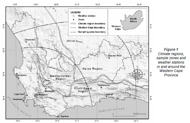
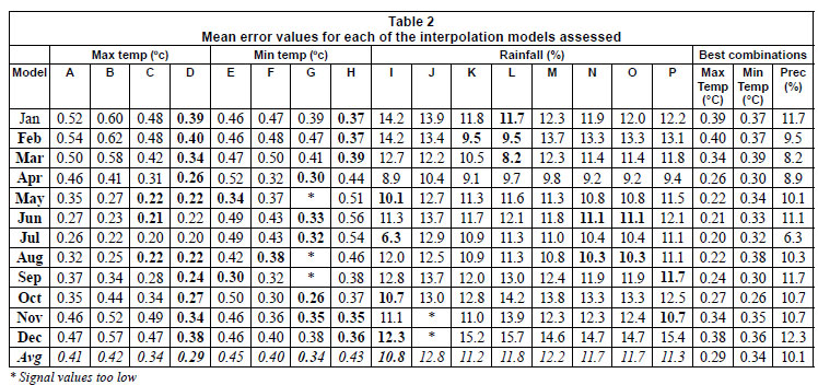
The first interpolation set (A in Table 1) for monthly mean daily maximum temperatures was generated using sampled monthly mean daily maximum temperature data, latitude, longitude, and elevation as input. The results (Table 2) show that an overall error of 0.41ºC is achieved when only latitude, longitude and elevation are incorporated as independent variables. Adding distance to oceans as an untransformed additional variable (Model B) did not improve overall accuracy, although some improvements were observed for months April to September. However, a significant (21%) improvement in overall accuracy was achieved when a natural logarithm is used to transform distance to oceans (Model C). When distance to oceans is scaled to kilometres prior to applying the logarithmic transformation (Model D), the overall error is further reduced to 0.29ºC - a 29% improvement compared to Model A. Apart from June, which had a slightly higher mean error than Model D, all of the monthly interpolations were more accurate than those of the other models used for interpolating maximum temperature. This suggests that distance to oceans has a significant influence on maximum daily temperatures in the Western Cape, but that its impact is restricted to a relatively narrow band along the coast.

 

 

 

Monthly mean daily minimum temperature

Distance to oceans also improved interpolations of monthly mean daily minimum temperature interpolations. Table 2 shows that overall error is reduced from 0.45ºC (Model E) to 0.4ºC when untransformed distance to oceans is incorporated (Model F). An additional improvement of 0.06ºC is achieved when distance to oceans is transformed using the natural logarithm (Model G). Although no interpolations were possible for May, August, and September (due to low signal values), Model G produced the most accurate surfaces for April, June, July, October and November. Scaling distance to oceans to kilometres prior to transformation (Model H), produced the most accurate interpolations for January, February, March, November and December, but resulted in higher overall mean error values than Models F and G. From these results it is clear that no single set of input variables is superior for interpolating monthly mean daily minimum temperature and that a combination of models will be required to develop the most accurate surface set.

 

Monthly mean rainfall

For monthly mean rainfall interpolations, 8 combinations of input variables provided results that had signal values of less than 80% and overall error margins of less than 30% (see Table 2). The first interpolation set (Model I) considered latitude, longitude and elevation during interpolation and produced an overall error margin, expressed as a percentage of maximum monthly rainfall, of 10.8%. This error is at the lower extreme of the 10-30% error-margin range suggested by Hutchinson et al. (1996). Introducing distance to oceans as a fourth input variable (Model J) increases overall error to 12.8%, although the mean errors of the January through March interpolations improved slightly compared to Model I. Further improvements for these months, as well as August, September and November, are achieved when distance to oceans is transformed logarithmically (Model K). Scaling distance to oceans to kilometres before logarithmic transformation (Model L) improved the accuracies for January and March, but reduced overall accuracy slightly.

Substituting distance to oceans with hillshade (Model M) also did not improve overall accuracy (compared to previous models), but superior accuracies were achieved for June, August and September when hillshade was scaled (multiplied by 10) prior to interpolation (Model N) or when transformed using a logarithmic equation (Model O). The investigation into the effect of different input variables for interpolating mean monthly rainfall concluded with Model P in which both distance to oceans and hillshade were used as input. The results show that this combination delivered superior interpolations for only 2 months (September and November). However, in spite of attempts to use various scaling and transformation techniques in the input variables, the maximum rainfall error values of the 5-variable interpolation sets (including Model P) were unrealistically higher (50%) than the recorded maximum error values. Given these results it can be concluded that the use of distance to oceans and topography as additional variables does not improve the overall interpolation accuracy of rainfall surfaces in the Western Cape.

The accuracy assessment was used to identify the input variables that produced the most accurate climate surface for any given month (highlighted in Table 2). To produce the final climate surfaces, the variables that produced the best results for any given month were used to interpolate new monthly surfaces using the full set of the weather stations (including the 20% sample that was used for the accuracy assessment) as input. The overall mean error for each data set was calculated by averaging the monthly mean errors of the selected surfaces in Table 2. Consequently, the overall mean error of the resulting rainfall surfaces is estimated to be 10.1%, while the mean error of the minimum and maximum temperature surfaces is 0.29ºC and 0.34ºC, respectively. This is, however, a conservative estimation since it reflects the accuracy of the interpolations sets that were generated from an incomplete (80%) set of input data.

 

Pair-wise comparison to existing climate surfaces

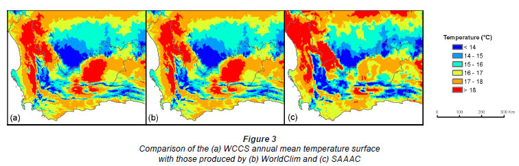
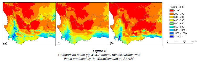
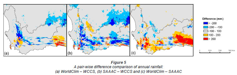
The monthly climate surfaces were used to compose mean temperature (Fig. 2a) and annual rainfall (Fig. 3a) surfaces for the Western Cape. At first glance, the resulting annual rainfall surface, shown in Fig. 2(a), seems very similar to the corresponding WorldClim and SAAAC surfaces (Figs. 2b and 2c, respectively). However, the pairwise difference maps (Fig. 4) reveal a number of deviations. When the WCCS annual rainfall surface is compared with WorldClim (Fig. 4a), the values of the WCCS surface is generally higher in the high, mountainous regions. This positive difference is even more pronounced in Fig. 4b, which pair-wise compares the WCCS annual rainfall surface to SAAAC. Although annual rainfall in excess of 2 000 mm is common in the Jonkershoek Mountains east of Stellenbosch, such high rainfall is unlikely to frequently occur in the Koue Bokkeveld Mountains north of Ceres. However, no rainfall stations are available in these high-altitude areas to verify this.

In contrast to the positive difference of rainfall in the mountainous regions, Ceres itself was interpolated to receive, on average, 591 mm of rainfall - considerably less than the WorldClim and SAAAC estimates of 949 mm and 976 mm, respectively. However, according to the records of the weather station in Ceres the actual long-term average is 567 mm, indicating that the WCCS surface is closer to the true rainfall. Similarly, the evident negative difference of rainfall values in the Worcester region (see Figs. 3a and 3b), were verified to be consistent with the long-term weather station records of Worcester.

Another area where there is a noticeable difference in interpolated annual rainfall is in the southern parts of the Cape Peninsula near Kommetjie. When compared to the 2 existing surfaces, it seems that the WCCS rainfall values are generally lower in this area. Closer inspection revealed that the WCCS interpolated value at Kommetjie is 572 mm, while the SAAAC and WorldClim values are 884 mm and 857 mm, respectively. However, the long-term average of annual rainfall at Kommetjie (Slanghoek) weather station is 466 mm, which indicates that all 3 interpolations overestimate rainfall, but that the WCCS interpolation is significantly more accurate in this area.

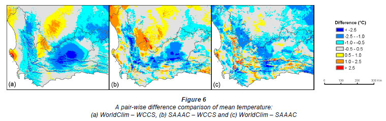
In terms of mean annual temperature, a significant (>2.5ºC) difference between the WCCS and WorldClim surface is apparent in the Saldanha region (see Fig. 5a). However, a similar pattern is observed in Fig. 5c, which suggests that it is the WorldClim surface that overestimates temperatures in this coastal region. Unfortunately, this could not be verified as no weather stations are available in this area (the nearest being Langebaanweg, which is about 13 km from Saldanha). Another area in which the WCCS temperature interpolation deviates significantly from WorldClim's is in the Tankwa Karoo and Hantam regions (Fig. 5a), but again there is no way to verify this, as the 2 weather stations that are present in those regions have been in operation for less than 5 years (and were consequently not included in the interpolation of the surfaces). However, the likelihood of a temperature underestimation in these areas is higher than in Saldanha because a similar, more pronounced, pattern is observed when WCCS is compared to SAAAC (Fig. 5b). In contrast to WCCS's relatively lower temperatures in the Tankwa Karoo, temperatures are relatively high in the south-western Karoo (compare Figs. 5a and 5b). However, the WCCS interpolated mean temperature at Prince Albert is 19.1ºC, which is consistent with the long-term mean temperature measurements at Prince Albert (19.6ºC). In contrast, the SAAAC and WorldClim interpolated temperatures are lower (16.9ºC and 15.8ºC, respectively) indicating that the WCCS interpolation is more accurate in the south-western Karoo region.

 

Resolution comparison to existing climate surfaces

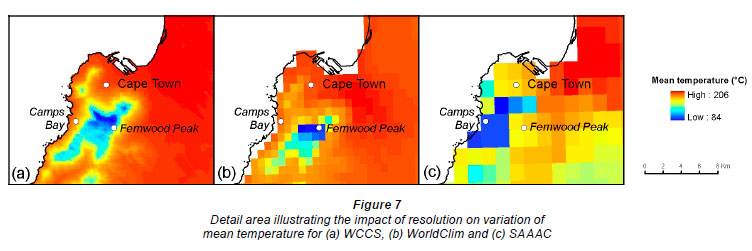
The value of WCCS's high resolution surfaces is only realised when they are compared to existing climate surfaces at large mapping scales. This is illustrated in Fig. 6, which shows the WCCS, WorldClim and SAAAC mean temperature surface of Cape Town. It is clear that the WCCS interpolation represents much more variation than the other 2 surfaces and that it has a higher horizontal accuracy. For example, according to Fig. 6c, the mean temperature at Camps Bay is lower than on Table Mountain at Fernwood Peak. This error is a direct consequence of the low resolution of the SAAAC surface (compare with Figs. 6a and 6b).

 

Figure 7

 

Conclusions

The research reported in this paper aimed to determine the best combination of input variables for interpolating climate surfaces in the Western Cape. When distance to oceans is introduced as an additional, transformed input variable for interpolating monthly mean maximum daily temperatures, the mean error was reduced by 29%. Clearly, ocean proximity is an important variable to include when interpolating monthly mean maximum daily temperatures in the Western Cape. Interpolation accuracy is also improved for the interpolation of the monthly mean minimum daily temperature for October through April when distance to oceans is used as an additional input variable. By contrast, distance to oceans has little effect on overall accuracy when included in monthly mean rainfall interpolations. Similarly, the inclusion of topography (represented by hillshade with an azimuth of 180º) did not improve overall interpolation of monthly mean rainfall. It did, however, produce more accurate rainfall surfaces for 4 months of the year (April, June, August and September).

Temporal (monthly) differences in interpolation accuracy were observed in most of the interpolation sets. This indicates that certain combinations of input variables are suitable for some months, but not for others. This observation was used to produce suitable interpolation sets by selecting and combining the input variables that produced the highest monthly accuracies.

Although most of the interpolation sets generated from the 80% sample of weather station data had a relatively low overall mean error, a pair-wise difference comparison of the re-interpolated surfaces (using all the meteorological data) with existing climate surfaces revealed some discrepancies. It seems that the WCCS surface overestimates rainfall in high-altitude regions, and underestimates temperatures in the Saldanha, Tankwa Karoo and Hantam regions. These differences could not be verified due to lack of reference data. However, in the areas where verification was possible (e.g. Ceres, Worcester, Kommetjie and Prince Albert), it was found that the WCCS interpolation was consistently more accurate than WorldClim and SAAAC.

In conclusion, this research showed that it is possible to improve climate surface interpolation accuracy by including elevation, distance to oceans, and hillshade as additional input variables and by selecting the most suitable input variable combinations on a monthly basis. Although a specific interpolation algorithm (ANUSPLIN) was used in this research, it is likely that the same combinations of input variables will also improve temperature and rainfall interpolations using other algorithms. More research is needed to determine if this is the case. Potentially, the combination of input variables evaluated in this research will improve climate surface interpolations in other parts of the world (although this will require further investigation), but for the Western Cape the higher resolution and accuracy of the newly-created surfaces will be of particular value for hydrological research.

 

Acknowledgments

We thank Michael Hutchinson, Australian National University, for his valuable advice and assistance with the operation of ANUSPLIN.

 

References

ARCHER E, CONRAD J, MÜNCH Z, OPPERMAN D, TADROSS M and VENTER J (2009) Climate change, groundwater and intensive commercial farming in the semi-arid northern Sandveld, South Africa. J. Integrative Environ. Sci. 6(2)139-155.         [ Links ]

BARRINGER JRF and LILBURNE LF (2000) Developing fundamental data layers to support environmental modeling in New Zealand: Progress and problems. URL: http://www.colorado.edu/research/cires/banff/pubpapers/221/ (Accessed 14 April 2011).         [ Links ]

BESAW LE, RIZZO DM, BIERMAN PR and HACKETT WR (2010) Advances in ungauged streamflow prediction using artificial neural networks. J. Hydrol. 386(1-4)27.         [ Links ]

BRADSHAW CJA, SODHI NS, PEH KSH and BROOK BW (2007) Global evidence that deforestation amplifies flood risk and severity in the developing world. Global Change Biol. 13(11)2379.         [ Links ]

BURROUGH PA and McDONNEL RA (1998) Principles of Geographical Information Systems. Oxford University Press, Oxford. 236 pp.         [ Links ]

CAREY VA (2005) The use of viticultural terroir units for demarcation of geographical indicators for wine production in Stellenbosch and surrounds. PhD dissertation, Stellenbosch University. 201 pp.         [ Links ]

CHANG KT (2010) Introduction to Geographic Information Systems, McGraw Hill, New York.         [ Links ]

CHAPMAN AD (2000) The case for a 3-minute climate surface for South America. Internal Report No. 3. Australian Biodiversity Information Services. 8 pp.         [ Links ]

FARAN ALI K and DE BOER DH (2008) Factors controlling specific sediment yield in the upper Indus River basin, northern Pakistan. Hydrol. Processes 22(16)3102.         [ Links ]

FOURIE JC (2006) Evaluating agricultural potential of a Cape Metropolitain catchment: A fuzzy logic approach. MSc thesis, Stellenbosch University. 73 pp.         [ Links ]

FUNK VA and RICHARDSON KS (2002) Systematic data in biodiversity: Use it or lose it. Syst. Biodiversity 51(2)303-316.         [ Links ]

HARTKAMP AD, DE BEURS K, STEIN A and WHITE JW (1999) Interpolation techniques for climate variables. Report No. 99-01. International Maize and Wheat Improvement Centre. 27 pp.         [ Links ]

HIJMANS RJ, CAMERON SE, PARRA JL, JONES PG and JARVIS A (2005) Very high resolution interpolated climate surfaces for global land areas. Int. J. Clim. 25 1965-1978.         [ Links ]

HOUGHTON JT, DING Y, GRIGGS DJ, NOGUER M, VAN DER LINDEN PJ, DA X, MASKELL K and JOHNSON CA (2001) Climate change 2001: The scientific basis. Cambridge Press, Cambridge. 881 pp.         [ Links ]

HUANG F and LI B (2010) Assessing grain crop water productivity of China using a hydro-model-coupled-statistics approach: Part I: Method development and validation. Agric. Water Manage. 97(7)1077.         [ Links ]

HUTCHINSON MF (1989) A new procedure for gridding elevation and stream line data with automatic removal of spurious pits. J. Hydrol. 106 211-232.         [ Links ]

HUTCHINSON MF (1998) Interpolation of rainfall data with thin plate smoothing splines - part II: Analysis of topographic dependence. J. Geogr. Inf. Decis. Anal. 2(2)152-167.         [ Links ]

HUTCHINSON MF (1998) Interpolation of rainfall data with thin plate smoothing splines: Part I. Two-dimensional smoothing of data with short-range correlation. Inf. Decis. Anal. 2(2)152-167.         [ Links ]

HUTCHINSON MF (2011) ANUSPLIN Version 4.3 [online]. Centre of Resource and Environmental Studies, Australian National University. URL: http://fennerschool.anu.edu.au/publications/software/anusplin.php (Accessed on 14 April 2011).         [ Links ]

HUTCHINSON MF, KALMA JD and JOHNSON ME (1984) Monthly estimates of wind speed and wind run for Australia. Int. J. Clim. 4(3)311-324.         [ Links ]

HUTCHINSON MF, NIX HA, MCMAHON JP and ORD KD (1996) The development of a topographic and data climate database for Africa. Proc. of the Third International Conference/Workshop on Integrating GIS and Environmental Modeling, NCGIA, Santa Barbara, California. URL: http://www.ncgia.ucsb.edu/conf/SANTA_FE_CD-ROM/santa_fe.html        [ Links ]

JAKOB D, TAYLOR BF and XUEREB KC (2005) A pilot study to explore methods for deriving design rainfalls for Australia - Report No. 10. Hydrometeorological Advisory Service, Bureau of Meteorology, Australia. 59 pp.         [ Links ]

JARVIS CH and STUART N (2001) A comparison among strategies for interpolating maximum and minimum daily air temperatures. Part I: The selection of guiding topographic and land cover variables. J. Appl. Meteorol. 40(6)1060-1074.         [ Links ]

JEFFREY SJ, CARTER JO, MOODIE KB and BESWICK AR (2001) Using spatial interpolation to construct a comprehensive archive of Australia climate data. Environ. Model. Software 16 309-330.         [ Links ]

LUTGENS FK and TARBUCK EJ (1998) The Atmosphere. Prentice Hall, New Jersey. 450 pp.         [ Links ]

LYNCH SD and SCHULZE RE (2006) Rainfall database. In Schulze RE (ed.) South African Atlas of Climatology and Agrohydrology. WRC Report No. 1489/1/06. Water Research Commission, Pretoria.         [ Links ]

McKENNEY D (2000) Development of gridded climate data for Canada and North America using thin plate splines. Canadian Forest Service (3-5 November 2000). 27 pp.         [ Links ]

PRICE DT, McKENNEY DW, NALDER IA, HUTCHINSON MF and KETSTEVEN JL (2000) A comparison of two statistical methods for spatial interpolation of Canadian monthly mean climate data. Agric. Forest Meteorol. 191 81-94.         [ Links ]

PRICE DT, McKENNEY DW, PAPADOPOL P, LOGAN T and HUTCHINSON MF (2004) High resolution future scenario climate data for North America. Proc. Amer. Meteor. Soc. 26th Conference on Agricultural and Forest Meteorology, 23-26 August 2004, Vancouver, BC. 13 pp.         [ Links ]

RODRIGUEZ E, MORRIS CS, BELZ JE, CHAPLIN EC, MARTIN JM, DAFFER W and HENSLEY S (2005) An assessment of the SRTM topographic products. Jet Propulsion Laboratory, Pasadena. 143 pp.         [ Links ]

SCHULZE RE (1997) South African Atlas of Agrohydrology and -Climatology. WRC Report No. TT 82/96. Water Research Commission, Pretoria. 276 pp.         [ Links ]

SCHULZE RE and MAHARAJ M (2006) Temperature database. In: Schulze RE (ed.) South African Atlas of Climatology and Agrohydrology. WRC Report No. 1489/1/06. Water Research Commission, Pretoria.         [ Links ]

SHARPLES JJ, HUTCHINSON MF and JELLETT DR (2005) On the horizontal scale of elevation dependence of Australian monthly precipitation. J. Appl. Meteorol. 44 1850-1865.         [ Links ]

SIEBERT S and DÖLL P (2010) Quantifying blue and green virtual water contents in global crop production as well as potential production losses without irrigation. J. Hydrol. 384(3-4)198.         [ Links ]

SOUTH AFRICAN WEATHER BUREAU (1996) Weather and climate of the extreme south-western Cape. Department of Environmental Affairs and Tourism, Pretoria. 39 pp.         [ Links ]

TAIT A, HENDERSON R, TURNER R and ZHENG X (2006) Thin plate smoothing spline interpolation of daily rainfall for New Zealand using a climatological rainfall surface. Int. J. Clim. 26(14)2097.         [ Links ]

UNITED STATES GEOLOGICAL SURVEY (2006) Shuttle Radar Topography Mission DTED. URL: http://edc.usgs.gov/products/elevation/srtmdted.html (Accessed 10 February 2006).         [ Links ]

VAN NIEKERK A (2008) CLUES: A web-based land use expert system for the Western Cape. PhD dissertation, Stellenbosch University. 221 pp.         [ Links ]

VICENTE-SERRANO SM, SAZ-SÁNCHEZ MA and CUADRAT JM (2003) Comparative analysis of interpolation methods in the middle Ebro valley (Spain): Application to annual precipitation and temperature. Clim. Res. 24 161-180.         [ Links ]

WASSENAAR LI, VAN WILGENBURG SL, LARSON K and HOBSON KA (2009) A groundwater isoscape for Mexico. J. Geochem. Explor. 102(3)123.         [ Links ]

WINTER K (2002) Oxford Intermediate Atlas of Southern Africa (in Afrikaans), Oxford University Press, Cape Town. 64 pp.         [ Links ]

ZHU Q, JIANG H, LIU J, WEI X, PENG C, FANG X, LIU S, ZHOU G, YU S and JU W (2010) Evaluating the spatiotemporal variations of water budget across China over 1951-2006 using IBIS model. Hydrol. Proc. 24(4)429.         [ Links ]

ZUO H, HUTCHINSON MF, McMAHON JP and NIX HA (1996) Developing a mean monthly climatic database for China and Southeast Asia. In: Booth TH (ed.) Matching Trees and Sites. ACIAR Proceedings, Canberra.         [ Links ]

 

 

Received 20 October 2010; accepted in revised form 30 May 2011.

 

 

* To whom all correspondence should be addressed. +2721 808-3101; fax: +2721 808-3109; e-mail: avn@sun.ac.za