Theoretical and numerical analysis of the influence of the bottom friction formulation in free surface flow modelling

 

 

O Machiels^*; S Erpicum; P Archambeau; B Dewals; M Pirotton

HACH Unit, ArGEnCo Department, University of Liège, Chemin des chevreuils 1-B52/3, 4000 Liège, Belgium

 

 

---

ABSTRACT

Bottom friction modelling is an important step in river flow computation with 1D or 2D solvers. It is usually performed using energy slope based formulations established for uniform flow conditions, or using a turbulent regime based approach relying on turbulence analysis. However, these formulations are often applied under conditions of relative roughness which lie far outside of their validity fields. Furthermore, the theoretical definition of the roughness coefficients, defined by the different authors of both approaches, is not valid for usual numerical flow modelling, considering numerical approximations. The value of this coefficient becomes generally dependent on the flow conditions. Following the definition of the flow validity field of the main friction formulations proposed in literature, an original formulation has been developed. It combines 2 explicit turbulent regime based formulations smoothly linked by a polynomial expression, providing a continuous formulation covering the wide range of roughness usually encountered in river flows. The formulation is suitable to model, with a unique value of the friction coefficient, river flows with a wide range of hydrodynamic properties (water depth, discharge). The efficiency of this new formulation, fitted to explicit friction formulations and numerically adjusted, is demonstrated through various 1D and 2D practical applications.

Keywords: friction, river flow, modelling

---

 

 

Introduction

Shallow-water equations are commonly used to numerically model river flows (Erpicum et al., 2010). Indeed, the main assumption of these equations is that the flow velocity component normal to the main flow plane is smaller than the flow velocity components in this plane. This is the case for the majority of river flows where the vertical velocity component is negligible compared to horizontal ones, except in the vicinity of singularities such as weirs, for example. this paper focuses on bottom friction modelling in mathematical models based on these shallow-water equations. The effect of bottom friction is of great importance for real flow computation, despite the fact that flow is generally evaluated from energy slope based formulations experimentally determined for uniform flow conditions.

The bottom friction term should represent the whole of the energy losses induced by flow resistance on the rough river bed. It is thus related to the bed characteristics (shape, roughness), to the fluid characteristics (viscosity) and to the flow features (water height, velocity, shear stress) (Morvan et al., 2008; Verbanck, 2008).

The concept of friction slope (Carlier, 1972) was already used over 3 decades ago to characterise bottom friction. The friction slope is a non-dimensional number corresponding to the slope of a prismatic channel where a uniform flow establishes for a given discharge. This concept was the basis for the first friction formulations proposed in the second part of the 18^th century, by the researchers of the so-called 'energy slope based' school. Authors such as Chezy (Mouret, 1921) and Manning (1890) proposed similar formulations based on results of experiments consisting of measuring the friction slope for a number of idealised flows in a laboratory flume. A second approach appeared later following works of Prandtl (1904). It provided formulations issued from analysis of the physics of the shear layer phenomena, referred to as the 'turbulent regime based' school.

Today, both approaches are used by free surface flow modellers, and these formulations are sometimes applied to flow conditions far removed from those upon which the approaches were originally based. It is thus important to keep in mind the validity ranges for each of these formulations and to note the lack of a single formulation able to describe the bottom friction phenomena for largely variable flow conditions.

Furthermore, other effects affecting the flow energy, which can either be linked to the bottom roughness, such as those due to turbulence, or be independent, such as wind effects, are included in the friction term used by most flow solvers (Morvan et al., 2008). In this case, it is then important to keep in mind that the friction slope terms in mathematical models do not only represent the direct bottom friction phenomenon.

The aims of the work presented in this paper were to define the validity fields of various bottom friction formulations proposed in literature, and to find and validate an original continuous formulation for bottom friction computation in river flow solvers.

 

Usual friction formulations

Energy slope based formulations

The formulations of the so called 'energy slope based' school have all been developed on the basis of experimental tests. These tests consisted of measuring the slope of a prismatic channel where a uniform flow can be obtained (Carlier, 1972). In these flow conditions, simple formulae can be set up to link the channel roughness, the flow variables and the bottom slope. Replacing the bottom slope by the friction slope, the friction effects can be computed for flow conditions other than the uniform ones. The general form of energy slope based friction formulations is given by:

This relates the friction slope J to hydraulic and geometric parameters affecting the bottom friction, such as U, the mean flow velocity, α, a friction coefficient and R_h, the hydraulic radius. This last parameter reflects the effect of the cross sectional shape. The differences between the different friction formulations of the energy slope based school lie in the χ exponent value (Table 1) and in the α coefficient form.

 

 

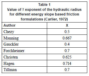
Chezy and Manning formulations are the most widely used energy slope based friction formulations because of the extensive knowledge of the friction coefficient, α, which is available in literature for both formulations (Bazin, 1865; Ganguillet and Kutter, 1869; Strickler, 1923; Barnes, 1967). It is important to note that these formulations do not explicitly take into account the turbulence regime of the flow, despite the fact that it is well known that this flow state has a great influence on the friction losses.

Turbulent regime based school

In contrast with energy slope based formulations, formulations from the turbulent regime based school rely on a sound theoretical background on the physics of the friction phenomena (Carlier, 1972). Under the leadership of Prandtl, researchers from the University of Göttingen (Germany) developed formulations of a friction coefficient, λ, depending on the turbulence state of the flow, through the Reynolds number, Re, and the size of the roughness elements of a pipe, k. turbulent regime based formulations were initially developed for pressurised flows to determine head losses in pipes. However, they can be extended to channel conditions considering an equivalent diameter 4R_h (Chadwick et al., 2004). These formulations thus remain applicable to free channel flows considering an equivalent Reynolds number Re related to the Reynolds number for free surface flows Re*:

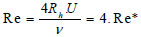
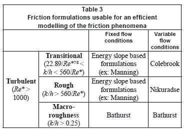
This paper focuses on the determination of the bottom friction term for river flow modelling. The form of the turbulent regime based formulations presented hereafter is thus the form valid for open channel flows, in which Re* is used. Usual river flow regimes are transitional, rough turbulent or macro-roughness regimes.

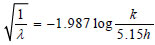
The Darcy-Weisbach equation (Weisbach, 1845) links the friction slope J to the friction coefficient λ:

In 2D flow modelling, the hydraulic radius R_h is equivalent to the water depth h. For the remainder of this paper both expres sions will be similarly used.

Rough turbulent regime

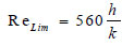
The rough turbulent regime is defined by a ratio between the Reynolds number, Re, and the relative roughness, k/h. Indeed, the more turbulent the flow, the smaller the laminar boundary layer and the more important is the effect of the wall roughness on friction formulations. The rough turbulent regime appears when the effects of the roughness are predominant, i.e. for values of the Reynolds number Re* higher than a limit value Re_Lim defined by (Carlier, 1972):

For this regime, Nikuradse (1933) developed an explicit formulation of the friction coefficient, λ, as a function of the relative roughness, k/h:

Transitional regime

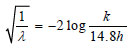
The transitional regime is the regime between the smooth and rough turbulent regimes. Colebrook (1939) proposed the following formulation of the friction coefficient:

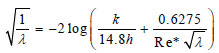
The implicit character of this equation makes its use difficult. Different authors developed explicit equivalent formulations (Barr, 1977; 1981; Yen, 1991). The second formulation of Barr provides the best results regarding the Colebrook formulation, with less than 1% error on the friction coefficient values in the corresponding range of Re* values. It is written as:

Macro-roughness

Macro-roughness is considered when the size of the roughness element k becomes comparable to the water depth h:

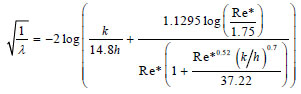
the formulation of Bathurst (1985) is a reference to study flows on macro-roughness:

 

Validity fields of the energy slope based formulations

On the one hand, the energy slope based formulations have not been developed with regard for the variation in turbulence regime which is found in real water flows. All of these formulations have been defined within the scope of specific applications and for fixed uniform flow conditions.

On the other hand, turbulent regime based formulations take the turbulence regime of the flow into account better, but none of them can be applied to the whole flow conditions of real river flows. Furthermore, the energy slope and turbulent regime based formulations are not similar for all values of the roughness (Henderson, 1966; Morvan et al., 2008).

In this section, the validity field of the main energy slope based formulations is defined by comparison with the friction loss values provided by the corresponding turbulent regime based formulations, depending on the flow turbulence regime.

Rough turbulent regime

In the rough turbulent regime, the Nikuradse formulation is a complex function of the water depth, h. Inserted in the Darcy-Weisbach equation, the turbulent regime based formulation cannot be compared directly with the energy slope based formulations. This problem can be solved by replacing the logarithm of the relative roughness by its power development (Dubois, 1998):

The energy slope based-like formulation of Nikuradse's equation is then obtained by conservation of the λ value and of its derivative with regard to k/hin the Darcy-Weisbach equation:

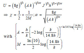
All energy slope based formulations using a χ exponent higher than 0.5 are thus equivalent to the Nikuradse formulation for a particular value of the relative roughness k/h. For χ = 0.5, the coefficient M value must be infinity, thus the relative roughness must be 0. So the Chezy's formulation is a limit to the bottom friction evaluation in turbulent regime in the case of a smooth bed. Formulations with a χ value lower than 0.5 are not valid in this specific flow regime.

In the Manning's formulation, with χ = 0.667, the value of M has to be 3. This means that the bottom friction is correctly evaluated for a relative roughness equal to 0.037. In this case, calculation of α is very close to the Strickler formulation (Strickler, 1923):

For other energy slope based formulations using an exponent χ higher than 0.5, the same calculations can be performed. Each of these formulations is thus suited to correctly describe the bottom friction phenomena for a specific value of the relative roughness and a particular form of the α coefficient, as shown in Table 2.

 

 

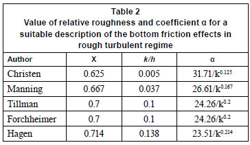
Considering the whole of the energy slope based formulations, the bottom friction in rough turbulent flows can be correctly evaluated for relative roughness up to 0.2. This last value is near the limit of macro-roughness. However, each formulation considered separately is only valid for a single relative roughness value, and none is thus available for general use.

Transitional regime

The same developments as for the Nikuradse's formulation can be performed with Colebrook's formulation in transitional regime. However, the coefficients A and M also become a function of the Reynolds number and thus of the turbulence state of the flow:

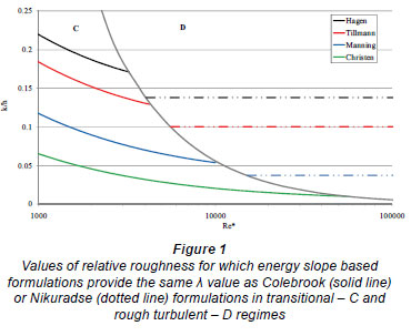
The Chezy formulation thus imposes a limit to the bottom friction evaluation in turbulent regime for smooth bed and the formulations with χ exponent value lower than 0.5 are not valid for a transitional regime. The other energy slope based formulations are valid for a single value of the relative roughness. However, this value varies with the Reynolds number as shown in Fig. 1.

 

 

As for the rough turbulent regime, the bottom friction value for transitional flows can be correctly evaluated with energy slope based formulations for specific flow conditions, but none of the formulations is of universal application.

Macro-roughness

For macro-roughness, the same reasoning can be applied as for the rough turbulent regime. Coefficients A and M are not a function of the Re* value:

As no energy slope based formulation is valid for relative roughness higher than 0.2, none is applicable to macro-roughness.

Summary

As a result of the study described above, a choice of friction formulation for free surface flow modelling could be made, depending on the flow conditions (Table 3) (Machiels, 2008). Due to the time cost of the computation of implicit formulations, explicit formulations are preferred, when they are available, to correctly describe the friction phenomena.

 

 

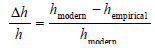
To define more precisely the validity fields of the different energy slope based friction formulations compared to the turbulent regime based ones, it is necessary to define the error for friction loss evaluation for both approaches:

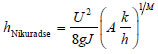
For example, considering the Nikuradse's formulation, the water depth is computed as:

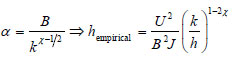
Regarding the study of the rough turbulent regime (Table 2), coefficient α could be expressed as a function of the roughness only (B is a constant parameter). The water depth computed by the energy slope based formulations can then be evaluated, using:

Combining these formulations, the error depends only on the relative roughness. Validity fields of the friction formulations for the description of rough turbulent regime can thus be defined in terms of relative roughness (Machiels, 2008).

Applying the same reasoning for transitional regime and for macro roughness and considering an acceptable relative error of 5%, the validity fields of the different energy slope based friction formulations can be extended (Table 4). The boundary values of these validity fields are actually a function of the Reynolds number. However, the variations are negligible for usual values of Reynolds for river flows (Re* > 5000).

 

 

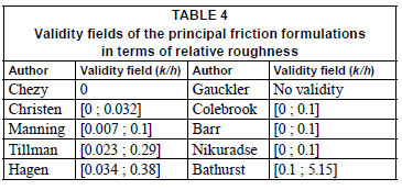
As a result of the comparison between modelling results and in situ measurements in river, as presented hereafter, the limit of the validity range of the macro-roughness formula has been extended to a relative roughness of 0.1.

Continuous friction formulation

Regarding the validity fields of the energy slope based and turbulent regime based formulations shown in Table 4, it is remarkable that a single formulation does not exist which is suited to computing friction effects across the whole range of relative roughness encountered in real river flows, where h ranges from 0 on the banks to several meters mid-channel, with an essentially constant roughness height k.

Furthermore, the definition of the friction coefficients α or k in the 1D and 2D traditional flow solvers does not correspond to the one given by the original authors of the friction formulations computed. Other effects affecting the flow energy, which can either be linked to the bottom roughness, such as those due to the turbulence, or be independent, such as numerical scheme effects, are included in the friction term used by most flow solvers (Morvan et al., 2008). The definition of the friction coefficient is thus a challenging problem for the correct computation of energy losses. Several authors have proposed formulations for these coefficients depending on the flow conditions and on the flow solver (Van Rijn, 1984; 2007; Morvan et al., 2008).

However, the turbulent regime based formulations have been developed based on the same definition of k for different ranges of relative roughness. Furthermore, the k/h validity ranges of several formulations are contiguous, such as, for example, for Colebrook or Barr and Bathurst.

Therefore, an original approach has been developed on the basis of the 4 following fundamentals:

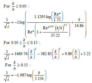
• Barr formula applies for turbulent flows with relative roughness k/h lower than 0.1

• Bathurst formula applies to compute friction effect on macro-roughness, i.e. for k/h higher than 0.1

• These 2 formulations are not equal for a relative roughness k/h in their respective validity fields

• The 2 formulations are developed based on the same definition of k, according to a unique value of the coefficient for particular river computing conditions (shape, flow, solver)

Developments have been performed to overcome the third point by continuously linking the 2 formulations close to relative roughness k/h equal to 0.1 (Machiels, 2008). Due to its explicit expression, Barr's formulation has been preferred to Colebrook's one.

To link the formulations of Barr and Bathurst, a third degree polynomial expression of the relative roughness has been set up:

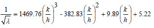
The limits of the application range of the different formulations have been chosen to ensure that the percentage of variation of the λ coefficient stays lower than 0.5 for a water depth variation of 1 cm. Thus the polynomial expression has been developed for k/h values between 0.05 and 0.15.

The parameters have been determined to get a continu ous variation of λ (same value and tangent) between the polynomial, the Barr and the Bathurst expressions at each limit of k/h range. These parameters are thus the solution of a 4 equation system depending on Re*. However, for Reynolds numbers Re* higher than 5000, which characterises most usual river flows, with k/h ratios in the range 0.05 to 0.15, the variation of the parameter values with Re* is negligible (less than 3% error on the 1/√λ value, Fig. 2). The final form of the polynomial expression is thus established with the constant parameter values obtained from an infinite value of Re*.

 

 

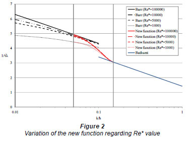
Combining the formulations of Barr and Bathurst with the new function provides an expression, which can be used to compute the bottom friction effects in rivers or channels, whatever the variation of k/h, for a unique value of k, depending on the river characteristics and on computing conditions. Although a discontinuity persists for k/h = 0.05 due to the Reynolds dependence of the Barr equation, the Barr and polynomial results remain sufficiently close to ensure the stability of the model if the Re* value is higher than 5 000. Furthermore, the flow solver used for validations hereafter forces the minimal value of Re* to be 5 000 in order to compute friction terms.

 

Validations

2D approach

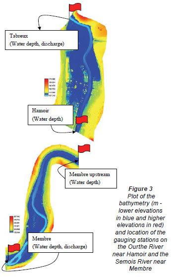
Two Belgian river reaches (gravel beds) were considered to validate the continuous approach: the first on the river Ourthe near the town of Hamoir and the second on the river Semois near Membre (Fig. 3). These 2 reaches, respectively 2.6 km and 1.6 km long, were selected because of the presence of 2 successive gauging stations on both of them. The downstream one combined with the discharge measurement provides the necessary boundary conditions for free surface flow numerical modelling (subcritical flows).

 

 

Both river reaches have been modelled using the 2D-horizontal finite volumes flow solver WOLF2D, developed at the University of Liege (Erpicum et al., 2010), using different friction formulations such as Manning, Barr, Bathurst and the continuous formulations, with a regular 2 x 2 m mesh.

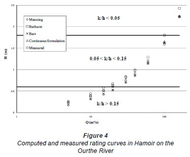
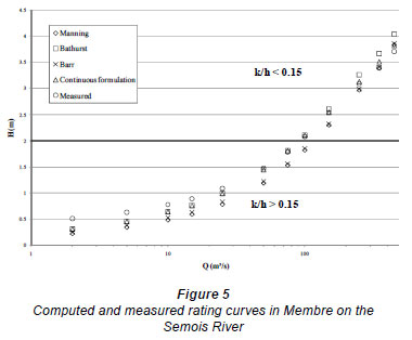
The comparison (Figs. 4 and 5; Table 5) between the upstream water depths computed using the formulations of Barr, Manning, Bathurst and the proposed continuous formulation, and the water depth measurements at the upstream gauging station for different discharges, have been used to highlight the value of the continuous formulation. It must be noted that the total computation time remains similar whatever the considered friction formulation.

 

 

 

 

 

 

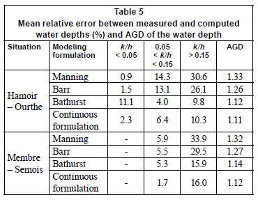
The average geometric deviation (AGD) of the water depth, proposed in Table 5, allows a classification of the different formulas' efficiencies. This was calculated, based on the measured h_m and the computed h_c water depth, as defined by Wu etal. (2008):

The Manning's coefficient n value was fitted regarding the real data for the highest discharge (Erpicum et al., 2010). It is equal to 0.025 s/m^1/3 in the Ourthe and to 0.031 s/m^1/3 in the Semois. The constant k value for Barr, Bathurst and continuous formulations was set up to get close to the measurements for both the lowest discharge with the Bathurst formulation and the highest discharge with the Barr equation. This value was 0.09 m in the Ourthe and 0.3 m in the Semois. These values are only issued from a calibration of the models. Indeed, as shown by Morvan et al. (2008), the value of these coefficients for numerical modelling differs from the empirical values proposed in literature (Van Rijn, 1984; 2007; Verbanck, 2008). The value of the proposed formulation is that it permits the representation of energy losses with a unique value of the friction coefficient k, for a particularly wide range of discharge and water depth.

The water depths are not homogeneous along the river reaches. The k/h ratio indicated in Table 5 is thus the ratio value at the upstream limit of the reaches, at the centre of the cross section. This is the reason why the results provided by the continuous formulation are not exactly equivalent to those provided by the Barr and Bathurst formulations, respectively, for k/h < 0.05 and k/h > 0.15.

On the Ourthe River, for k/h ratios lower than 0.05, the water depths computed using Manning, Barr and continuous formulations are relatively close to the measurements (less than 2.5%), whereas Bathurst results are less satisfactory (more than 10% error). This expresses well the validity of Barr and continuous formulations for 2D free surface flow modelling with low relative roughness. This also expresses the efficiency of the Manning formulation for flow conditions near those used in its development. Finally, this confirms that the Bathurst formula does not apply for low relative roughness, as shown in Table 4.

For k/h ratios higher than 0.15, the water depths provided using the Bathurst and continuous formulations are the closest to the measured values. The important value of the relative error is partially due to the effect of measurement uncertainty for low water depths. Indeed, water depth measurement accuracy is close to 5 cm in these cases. However, the results show the value of Bathurst and continuous formulations, compared to Manning and Barr ones, for flow modelling with high relative roughness. They also indicate the limitations of the Barr formulation for high relative roughness and of the Manning formulation when flow conditions differ from those used in its development.

For intermediary k/h ratios, the Bathurst formulation remains attractive when water depth has low variability on the river reach, such as on the Ourthe River. However, when water depth is more variable, such as on the Semois River, the continuous formulation becomes more accurate.

1D approach

Based on water depth and discharge measurements and considering a uniform flow, Martiny (1995) determined the K coefficient of the Manning-Strickler equation for a number of Belgian rivers. The uniform flow hypothesis is inaccurate for low water depths, but it becomes suitable for a larger river section. From Martiny's results, 6 cases, corresponding to the largest rivers studied, have been considered: the Sure River in Martelange, the Messancy River in Athus, the Vire River in Ruette, the Aisne River in Bomal-Juzaine and the Ourthe River in Amberloup and in Wyompont. For these 6 places, Martiny calculated K values depending on the water depth.

To compare Martiny's results with those provided by the proposed continuous formulation, the Strickler coefficient was expressed as a function of the friction coefficient λ. This was obtained by insertion of the Manning equation in the Darcy-Weisbach equation:

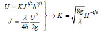
Considering the λ value provided by the proposed continuous formulation, this equation gives the value of the Strickler coefficient to use for an exact modelling of the continuous friction formulation. Figure 6 shows the comparison between Martiny's results and those provided by this equation, considering a unique bottom roughness for each river reach in the continuous formulation.

 

 

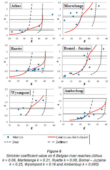
The mean relative error on the h value provided by the continuous formulation remains lower than 15% for all river reaches, except in Martelange, for water depth corresponding to macro-roughness. this comparison thus highlights the ability of the continuous formulation to describe the friction phenomenon for 1D flow modelling with a single roughness value, whatever the flow conditions (water depth, discharge), while the Manning formulation with a single K value is only suited to model the friction for a particular flow.

 

Conclusion

Friction is a complex phenomenon dissipating energy in water flows and thus strongly influencing water depths and flow velocities. It is thus necessary to take friction into account for correct flow modelling. Many authors have thus developed friction formulations, but these formulations are not always suited to describe the friction phenomenon across the whole range of real flow conditions.

The energy slope based formulations of Manning and Chezy are currently the most widely used formulations for friction modelling. This success stems from their explicit form and the extensive literature which exists on their parameter values. However, the turbulent regime based formulations are more representative of the physics of bottom friction. Furthermore, explicit forms of the turbulent regime based formulations exist, such as that of Barr. The turbulent regime based formulations thus have important value for flow modelling.

In practice, other effects on the flow energy, which can either be linked to the bottom shape (vegetation, bedforms, roughness), such as those due to turbulence, or be independent, such as wind effects, are included in the friction term used by most flow solvers. In this case, it is then important to keep in mind that the friction coefficients used in river flow solvers do not only represent the direct bottom friction phenomenon.

In this study, a determination of the different application ranges of the principal formulations has been proposed. In parallel, the validity fields of these formulations have been calculated in terms of relative roughness to correctly describe usual river flows.

An original friction formulation has also been developed in response to the lack of a continuous formulation able to describe the friction phenomenon for the highly variable flow conditions often encountered in river flows. This formulation combined the explicit formulation of Barr, available in turbulent regime, and that of Bathurst, available for macroroughness, smoothly linked by a polynomial expression of the relative roughness. The formulation so developed allows a continuous representation of the energy losses based on a unique definition of the roughness coefficient whatever the flow conditions (flow depth, discharge).

The formulation has been validated for 2D modelling by comparison of water depth values on 2 different river reaches in Belgium and for 1D modelling by comparison of experimental investigations on 6 Belgian river reaches. In both cases, considering a unique calibration of the friction coefficient of each reach, the continuous formulation enhances the representation of energy losses compared to other friction formulations (Manning, Barr, Bathurst) in general use.

 

References

BARNES HH (1967) Roughness Characteristics of Natural Channels. U.S. Geological Survey Water-Supply Paper 1849. United States Government Printing Office, Washington.         [ Links ]

BARR D (1977) Discussion of 'Accurate explicit equation for friction factor'. J. Hydraul. Div. 103 (3) 334-337.         [ Links ]

BARR D (1981) Solution of the Colebrook-White functions for resistance to uniform turbulent flows. Proc. Inst. Civ. Eng. 71 (2) 529-535.         [ Links ]

BATHURST JC (1985) Flow resistance estimation in mountain rivers. J. Hydraul. Eng. 111 (4) 625-643.         [ Links ]

BAZIN H (1865) Recherches Expérimentales sur l'Ecoulement de l'Eau dans les Canaux Découverts. in Mémoires présentés par divers savants à l'Académie des Sciences 19 1-494. Paris, France.         [ Links ]

CARLIER M (1972) Hydraulique Générale et Appliquée. Eyrolles, Paris. 565 pp.         [ Links ]

CHADWICK A, MORFETT J and BORTHWICK M (2004) Hydraulics in Civil and Environmental Engineering. Taylor & Francis, London. 603 pp.         [ Links ]

COLEBROOK CF (1939) Turbulent flow in pipes with particular reference to the transition region between the smooth and rough pipe formulations. J. Inst. Civ. Eng. 11 (4) 133-156.         [ Links ]

DUBOIS J (1998) Comportement hydraulique et modélisation des écoulements de surface. Communication 8, Laboratoire de Constructions Hydrauliques, Ecole Polytechnique Fédérale de Lausanne, Switzerland.         [ Links ]

ERPICUM S, DEWALS BJ, ARCHAMBEAU P, DETREMBLEUR S and PIROTTON M (2010) Detailed inundation modelling using high resolution DEMs. Eng. Appl. Comp. Fluid Mech. 4 (2) 196-208.         [ Links ]

GANGUILLET E and KUTTER WR (1869) Versuch zur Augstellung einer neuen allgeneinen Formel für die gleichformige Bewegung des Wassers in Canalen und Flussen. Zeitschrift des Osterrichischen Ingenieur - und Architecten-Vereines 21 (1 and 2) 6-25; 46-59.         [ Links ]

HENDERSON FM (1966) Open Channel Flow. The Macmillan Company, New York. 522 pp.         [ Links ]

MACHIELS O (2008) Analyse théorique et numérique de l'influence de la formulation des termes de production et de dissipation dans les équations d'écoulement à surface libre. Travail de fin d'études, University of Liege, Belgium.         [ Links ]

MANNING R (1890) On the Flow of Water in Open Channels and Pipes. Institute of Civil Engineers of Ireland.         [ Links ]

MARTINY A (1995) Contribution à la détermination du coefficient de rugosité des rivières. Ministère de la région wallonne, Direction des cours d'eau non navigables, Namur, Belgium.         [ Links ]

MORVAN HP, KNIGHT DK, WRIGHT NG, TANG X and CROSS-LEY AJ (2008) The concept of roughness in fluvial hydraulics and its formulation in 1-D, 2-D and 3-D numerical simulation models. J. Hydraul. Res. 46 (2) 191-208.         [ Links ]

MOURET G (1921) Antoine Chézy: histoire d'une formule d'hydraulique. Annales des Ponts et Chaussées 61 165-259.         [ Links ]

NIKURADSE J (1933) Strömungsgesetze in rauhen Rohren. VDI-Forschungsheft 361.         [ Links ]

PRANDTL L (1904) Über Flüssigkeitsbewegung bei sehr kleiner Reibung. Proc. 3rd Int. Math. Congr., Heidelberg, Duitsland.         [ Links ]

STRICKLER A (1923) Beiträge zur Frage der Geschwindigkeitsformel und der Rauhigkeitszahlen für Ströme, Kanäle und geschlossene Leitungen. Proc. of Eidgenössischen Amtes für Wasserwirtschaft, Bern, Switzerland.         [ Links ]

VAN RIJN LC (1984) Sediment transport, part III: bed forms and alluvial roughness. J. Hydraul. Eng. 110 (12) 1733-1754.         [ Links ]

VAN RIJN LC (2007) Unified view of sediment transport by currents and waves. 1. Initiation of motion, bed roughness, and bed-load transport. J. Hydraul. Eng. 133 (6) 649-667.         [ Links ]

VERBANCK MA (2008) How fast can a river flow over alluvium? J. Hydraul. Res. 46 (1) 61-71.         [ Links ]

WEISBACH J (1845) Lehrbuch der Ingenieur- und Maschinen-Mechanik. Braunschwieg.         [ Links ]

WU BS, VAN MAREN DS and LI LY (2008) Predictability of sediment transport in the Yellow River using selected transport formulas. Int. J. Sediment Res. 23 283-298.         [ Links ]

YEN BC (1991) Channel Flow Resistance: Centennial of Manning's Formula. Water Resources Publications, Highlands Ranch, Colorado. 454 pp.         [ Links ]

 

 

Received 1 February 2010; accepted in revised form 1 February 2011.

 

 

* To whomall correspondence should be addressed. Fund for education to Industrial and Agricultural Research (FRIA) +32 (0)4 366 95 96; fax: +32 (0)4 366 95 58; e-mail: omachiels@ulg.ac.be

 

 

Nomenclature

AGD	average geometric deviation
C	Chezy coefficient
g	acceleration of the gravity
h	water depth
J	friction slope
K	Strickler coefficient
k	roughness height
k/h	relative roughness
Re	Reynolds number for pipes
Re*	Reynolds number for open channel
Rh	hydraulic radius
U	flow velocity
λ	friction coefficient
ν	cinematic viscosity