Soil - water relationships in the Weatherley catchment, South Africa

 

 

CW van Huyssteen^*; TB Zere; M Hensley

Department of Soil, Crop and Climate Sciences, University of the Free State, PO Box 339, Bloemfontein 9300, South Africa

 

 

---

ABSTRACT

Soil water content is influenced by soil and terrain factors, but studies on the predictive value of diagnostic horizon type for the degree and duration of wetness seem to be lacking. The aim of this paper is therefore to describe selected hydropedological soil-water relationships for important soils and diagnostic horizons in the Weatherley catchment. Daily soil water content was determined for 3 horizons in 28 profiles of the Weatherley catchment. These data were used to calculate annual duration of water saturation above 0.7 of porosity (AD ), which was correlated against other soil properties. Significant correlations (α = 0.05) were obtained between average degree of water saturation per profile and slope (R² = 0.24), coarse sand content (R² = 0.22), medium sand content (R² = 0.23), fine silt content (R² = 0.19), and clay content (R² = 0.38). AD per diagnostic horizon ranged from 21 to 29 d•yr^-1 for the red apedal B, yellow brown apedal B, and neocutanic B horizons; 103 d•yr^-1 for the orthic A horizons; and from 239 to 357 d•yr^-1 for the soft plinthic B, unspecified material with signs of wetness, E, and G horizons. A regression equation to predict AD from diagnostic horizon type (DH), clay to sand ratio (Cl:Sa), and underlying horizon type (DH ) gave: AD = -26.31 + 41.64 ln(Cl:Sa) + 35.43 DH + 13.73 DH (R² = 0.78).Results presented here emphasise the value of soil classification in the prediction of duration of water saturation.

Keywords: diagnostic horizon, model, slope, soil texture, water saturation

---

 

 

Introduction

Van der Watt and Van Rooyen (1995) define soil water regime as a qualitative term referring to the state and availability of water in soil, especially in relation to the growth of plants. Another widely used, related, and probably more process-oriented and quantitative term, is soil hydrology. Miyazaki (1993) suggested that soil hydrology could be considered as a bridge between soil physics (where descriptions of water flow tend to be microscopic) and hydrology (where they tend to be macroscopic). Kutilek and Nielsen (1994) defined soil hydrology as the physical interpretation of phenomena which govern hydrological events related to soil, or the uppermost mantle of the earth's crust. Although both terms described above refer to soil-water relationships, neither are completely appropriate for the hydropedological focus of this study or the one by Van Huyssteen et al. (2005). The focus here was specifically on the nature of the long-term water content above the drained upper limit and the marked influence it may have on soil morphology and therefore soil classification.

Soil water content is mainly a function of the ratio between precipitation and evapotranspiration, as described by the soil water balance equation (Hillel, 1980). In general, the higher the rainfall to evapotranspiration (P/ET) ratio, the higher the soil water content. At a given site the soil water content varies depending mainly on variations in the topography, the soil, and the type and density of vegetation (Famiglietti et al., 1998). In a small catchment the rainfall can be considered fairly uniform over the whole area, although ET can vary significantly (Van Huyssteen et al., 2009a). Le Roux et al. (2005) concluded that the vegetation composition in the Weatherley catchment is fairly uniform and that the influence of vegetation on soil water content can therefore also be considered reasonably uniform. Soil and terrain characteristics should therefore be the primary factors that influence soil water content variability in this catchment.

Terrain indices can be grouped into primary and compound attributes. Primary terrain attributes (Famiglietti et al., 1998; Western et al., 1999) include:

• Slope, influencing the hydraulic gradient that drives surface and subsurface flow, surface runoff, infiltration, and drainage

• Aspect, together with slope, which influences the irradiance and thus evapotranspiration

• Plan curvature (perpendicular to the aspect) and profile curvature (parallel to the aspect) are measures of concavity or convexity of the surface. Plan curvature provides a measure of the local convergence or divergence of lateral flow paths, while profile curvature reflects how the hydraulic gradient and flow velocities change. Curvature is expressed as the reciprocal of the radius of curvature of the surface. Broader curves have smaller curvature values than tighter curves. Positive values indicate convex surfaces, zero indicates a straight surface, while negative values indicate concave surfaces.

• Specific upslope area, also called upslope contributing area, is the area above the contour segment divided by the length of that contour segment. It is a measure of the potential area that can contribute to lateral flow.

Terrain indices can be computed from digital elevation models (Mitasova and Hofierka, 1993). Compound indices, for example the wetness index (WI) defined by Beven and Kirkby (1979), can be calculated from primary topography attributes, and are often adapted, for example, the 'new index' (NI) for drier environments (Gomez-Plaza et al., 2001). The predictive power of terrain indices has been researched extensively, for example by Western et al. (1999), who did correlation analyses between terrain indices and soil water content in Australia. They defined the potential solar radiation index as the ratio of potential solar radiation on a sloping plane to that on a horizontal plane. During dry conditions cos(aspect) explained up to 12%, the potential solar radiation index explained up to 14%, and a combination of ln(α) and the potential solar radiation index explained up to 22% of the variance.

The influence of terrain indices on soil water content variability is often combined with other soil properties. Canton et al. (2004) and Lin et al. (2006) noted that it was difficult to identify the relative importance of the soil and topographic factors because of their mutual and multiple influences on soil water content. Soil factors include infiltration rate, water storage capacity, hydraulic conductivity, and the presence or absence of an impeding layer (Burt and Butcher, 1985). Gomez-Plaza et al. (2001) state that the influence of the soil factors studied on soil water content was different in the vegetated and non-vegetated zones and that the predictive power of WI was significantly increased by incorporating aspect (i.e. NI) and removal of slope, especially in unburnt catchments.

The relationship between soil properties and soil wetness has been studied in South Africa (Donkin and Fey, 1991; Le Roux, 1996; Van Huyssteen and Ellis, 1997; Van Huyssteen et al., 1997; Van Huyssteen et al., 2005) and in other countries (Rabenhorst et al., 1998; Blavet et al., 2000). Soil morphology contains significant information on the spatial and temporal distribution and circulation of water, both at profile and at landscape levels (Lin et al., 2005). Researchers used this information to predict soil wetness from soil morphology (Van Huyssteen and Ellis, 1997; Van Huyssteen et al., 1997; Rabenhorst and Parikh, 2000; He et al., 2003; Tassinari et al., 2002). These studies indicate that variability in soil water content is influenced by a combination of soil and terrain factors, and that the two are often inseparable. What has not yet been studied is the possible improvement to hydrological modelling that could be obtained by including the diagnostic horizon in the prediction of degree and duration of wetness.

The objective of this paper was to describe selected hydropedological soil-water relationships of selected soils and diagnostic horizons in the Weatherley catchment.

 

Materials and methods

Daily soil water contents were calculated using the procedure described by Van Huyssteen et al. (2009b). This included daily soil water contents for two to five, 300 mm layers of 28 soil profiles in the Weatherley catchment, for 6 years from 01 July 1997 to 30 June 2003. Profile numbers were defined to be distinctive within this catchment and also between other research catchments in the area (Hensley and Anderson, 1998). Profile numbers are used here in their original form to facilitate comparison. Soil water contents were expressed in terms of the degree of saturation (s), which is the fraction of the porosity that is occupied by water. Expressing soil water content as s enables comparisons between different soils and facilitates pedological interpretation. This point can be illustrated by considering 2 soils, say A and B, with bulk densities of 1.3 Mg•m^-3 and 1.7 Mg•m^-3 respectively. The volumetric water content (θ_v) for Soil A and Soil B at s = 0.7 would be 36% and 25%, and at complete saturation (s = 1.0) θ_v would be 51% and 36%, respectively. Reporting the θ_v values (51% and 36%) might give the impression that Soil A is wetter than Soil B, unless the bulk density (or porosity) values are also reported, while in reality both of them are completely saturated.

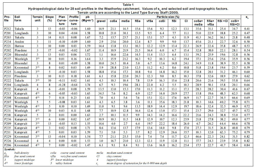
Detailed morphological soil profile descriptions, with chemical and physical analyses, are given by Van Huyssteen et al. (2005). Results for particle size analyses (Soil Classification Working Group, 1991) were averaged for the 0-900 mm depth and therefore no not necessarily add to 100%.

The s _s value for the different soils in the Weatherley catchment, as used here was defined as the mean daily s value of the 0-900 mm layer over the 6-year measurement period. There were only 2 profiles, P207 and P209, with measurements for the top 2 layers only. For these profiles the s_s values were taken over the 2 top layers. The s_s values of the different soils were compared with soil and topographic variables that might affect soil wetness. Mean daily s values for each month were also calculated for specific diagnostic horizons. These values aided in demonstrating the influence of the soil and topographic variables on s during different seasons.

Other hydropedological characteristics which were calculated for diagnostic horizons included the mean annual duration of s>0.7 (AD ), the mean annual frequency (F_s>0.7 ), and the mean duration (D_s>0.7 ) of periods with s>0.7 (Van Huyssteen et al., 2005). The 0.7 threshold was chosen as an estimation of where reduction would set in, because 100% water saturation is seldom reached (Hillel, 1980). The duration of s>0.7 for a particular year is the total number of days in that year on which s was above 0.7 of porosity. Whenever it occurs, the value s>0.7 could occur for periods of 1 day or longer. These periods are referred to as events. The frequency term (F_s>0.7 ) refers to the number of such events. The mean duration of events (D_s>0.7 ) is thus the ratio of the total number of days per year to the number of events per year. Due to their annual nature, a single value of each of AD_s>0.7 , F_s>0.7 and D_s>0.7 could be calculated per year during each of the 6 years of study for each diagnostic horizon. Their means were then calculated from the 6 annual values.

Only measurements that represented at least 80% of the volume of a particular diagnostic horizon were considered for this analysis. This was necessary to avoid possible erroneous conclusions introduced by measurements taken over transitions between diagnostic horizons. Terrain indices for the Weatherley catchment were calculated using ArcView 3.1 (ESRI, 1999). A 20 m grid-based digital elevation model was calculated, using kriging interpolation, from a 2 m interval contour map of the Weatherley catchment (BEEH, 2003).

Linear correlation analyses were done for diagnostic horizons between soil chemical, physical, and morphological properties and topographic indices as independent variables, with AD and mean monthly s for the 12 months as dependent variables. This was done in the form of a correlation matrix, with 70 observations of each variable. Prior to this, pair-wise scatter plots of independent and dependent variables were drawn to test the linearity of the relationships. In some cases it was necessary to transform the independent variable data to linearise the relationships. Qualitative data (diagnostic horizon and soil structure) were assigned dummy variables (Cody and Smith, 1997) to enable representation in the regression analyses. Eight different types of diagnostic horizons were available for the analyses. An integer between 1 and 8 was assigned to each of them in increasing order of their relative wetness based on their definitions (Soil Classification Working Group, 1991) and experience (Van Huyssteen et al., 2005). The numbering assigned was neocutanic B = 1, red apedal B = 2, yellow apedal B = 3, orthic A = 4, soft plinthic B = 5, E = 6, unspecified material with signs of wetness = 7, and G = 8. Saprolite, which was present underlying a diagnostic horizon in a single instance, was assigned 9. Soil structure was divided into 2 classes: massive, crumb, and granular were assigned 0, whereas subangular blocky, angular blocky, columnar, and prismatic were assigned 1.

The correlation matrix results helped to identify the strength of relationships between independent and dependent variables. These results also assisted in determining if relationships existed between independent variables, a situation that might lead to multi-collinearity problems and was therefore considered undesirable (NCSS, 1998; Fekedulegn et al., 2002).

Independent variables that correlated with AD_s>0.7 were further analysed using multiple linear regression analysis (NCSS, 1998) to identify their combined effect on AD_s>0.7. To reduce the number of variables to a manageable level, while at the same time keeping a sufficient number in the model, a procedure known as All Possible Regressions (NCSS, 1998) was used. This procedure helps to select the best number and combination of independent variables from the available options.

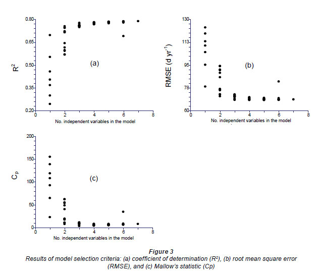
The most commonly used selection criteria (NCSS, 1998) are:

• Coefficient of determination (R²) - the larger the R² value, the better the model

• Root mean square error (RMSE) - the smaller the RMSE, the better the model

• Mallow's statistic (Cp) - in the optimum model the Cp value is close to p+1, where p is the number of independent variables. Deviation from this indicates that the model contains either too many or too few variables.

Multiple regression analysis was run on the independent variables selected according to the above-mentioned criteria. To use the resulting regression equation for prediction, the residuals (predicted - observed) must be independent of one another (Webster, 1997). This assumption was verified visually by plotting the residuals against each of the independent and dependent variables.

A test of the predictive capacity of the fitted regression model was conducted using a cross-validation procedure. This procedure, described by Wilks (1995), uses all observations (n) of the dependent variable (Y) for validation in a way that allows each observation to be treated, one at a time, as independent data. It regresses n-1 observations of Y on the corresponding observations of the predictors (X) to develop a regression equation. The equation is then used to predict the remaining i^th observation of Y from the X on row i. This is repeated for each observation (n times), producing n equations and therefore n predicted values. The final reported equation is fitted using all n observations. The advantage of this type of cross-validation procedure is that it avoids splitting the data into model development and validation data, thus yielding higher degrees of freedom. The statistical model evaluation procedures of Willmott (1981) were used to test the cross-validation results.

 

Results and discussion

The values of ss display a trend that was more-or-less consistent with the pedologically expected relative wetness levels of these soils (Fig. 1). At the drier end of the spectrum were the Tukulu, Hutton, Avalon, Pinedene, and Bloemdal soil forms, followed by Longlands and Westleigh soil forms and, towards the wet end, by the poorly drained Kroonstad and Katspruit soil forms.

 

 

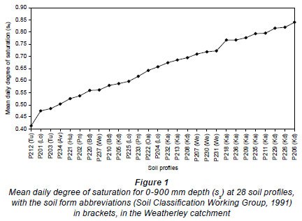
The increase in s_s (Table 1) was accompanied by a discernible change in topographic and soil characteristics. The terrain unit changed from primarily 3 to primarily 3⁽¹⁾, 4, and 5, while the slope angle generally decreased. Particle size distribution changed from primarily coarser for the drier soils to primarily finer for the wetter soils. Correlation analysis of the numeric values of the terrain and soil factors with s_s across the soils (n = 28) resulted in significant correlations (α = 0.05) for slope (R² = 0.31), coarse sand (coSa) content (R² = 0.28), medium sand (meSa) content (R² = 0.24), fine silt (fiSi) content (R² = 0.28), and clay (Cl) content (R² = 0.18). Other factors did not show significant correlation.

Monthly means of daily s values for each month of the year, averaged from the 6-year daily data and grouped per diagnostic horizon, are presented in Fig. 2. E horizons had the highest mean s, followed by G, unspecified material with signs of wetness, and soft plinthic B horizons.

 

 

Pedologically, one would expect the E horizons to be drier than the G horizons and unspecified material with signs of wetness (Soil Classification Working Group, 1991). However, this was not the case in this study. The discrepancy could be due to error introduced by the small number of E horizons (3), as compared to the G horizons (21) and unspecified material with signs of wetness (18), possibly causing bias. One of the E horizons was from P226 (Kd) and the other two were from P229 (Kd), both of which were very wet soils (Table 1). In both cases, the E horizons were underlain by G horizons which were wetter than the overlying E horizons. On average, the G horizons were, however, drier than the E horizons (Fig. 2). A significant contributing factor was probably the G horizons located in drier soils (Table 1) in the catchment e.g., P205 (Kd), P208 (Kd), and P232 (Ka).

Orthic A horizons were considerably wetter than the yellow brown apedal B, red apedal B and neocutanic B horizons during the summer (rain) months (December, January, February, and March). During the drier months of the year, however, the orthic A horizons were drier than the yellow brown apedal B and red apedal B horizons. This was expected, because orthic A horizons, being the upper horizons, have the greatest net water loss due to evapotranspiration (ET) during the rain-free winter months, while receiving most of the rainfall in summer months.

The yellow brown apedal B, red apedal B, and neocutanic B horizons decreased in wetness in the order: yellow brown apedal B > red apedal B > neocutanic B. These 3 horizons, as well as orthic A and soft plinthic B horizons, displayed considerable variations through the year, as opposed to the fairly constant wetness of the E and G horizons and unspecified material with signs of wetness. This reflected the extent of lateral and vertical drainage and losses due to ET from the orthic A and soft plinthic B horizons. The deeper and less permeable horizons lost less water through drainage and ET, while receiving more interflow water from higher-lying soils.

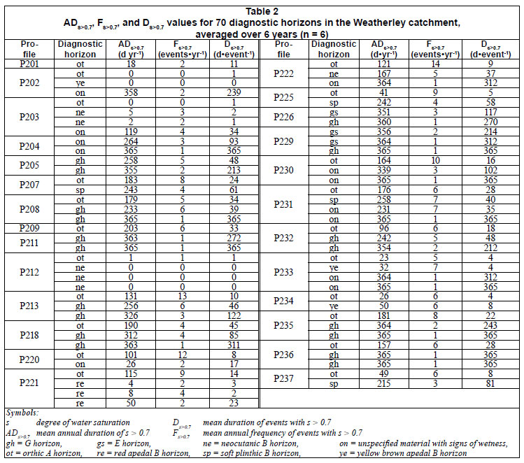
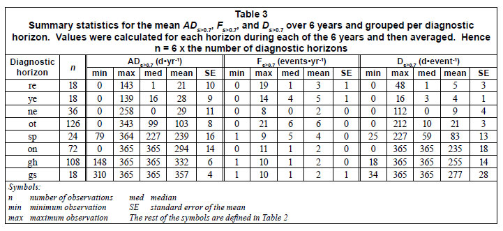
The AD_s>0.7 , F_s>0.7 and D_s>0.7 values for the diagnostic horizons are presented in Table 2. Summary statistics, averaged over 6 years and grouped by diagnostic horizon (Table 3), were done to facilitate comparisons of the variability of the values within and between diagnostic horizons. Mean AD_s>0.7 values ranged from 21 to 29 d•yr^-1 for the red apedal B, yellow brown apedal B, and neocutanic B horizons; 103 d•yr^-1 for the orthic A horizons; and from 239 to 357 d•yr^-1 for the soft plinthic B, unspecified material with signs of wetness, E, and G horizons. All 3 red apedal B horizons in this analysis (Table 3) were located in P221, which had a relatively wet orthic A horizon (AD_s>0.7= 115 d•yr^-1) and very dry red apedal B horizons (AD_s>0.7 < 50 d•yr^-1). The reason for this anomaly was not clear. The relatively high standard error for the neocutanic B horizons can be attributed to the relatively wet neocutanic B horizon (AD_s>0.7 = 167 d•yr^-1) at P222, compared to the drier neocutanic B horizons at P203 and P212 (AD_s>0.7 < 5 d•yr^-1). The AD_s>0.7 values in the yellow brown apedal B horizons ranged from 0 at P202 to 32 d•yr^-1 at P233 and 50 d•yr^-1 at P234, resulting in the high standard error.

The means of D_s>0.7 values (Table 3) were consistent with the morphology of the diagnostic horizons. All the diagnostic horizons which normally show considerable signs of wetness (i.e. soft plinthic B, unspecified material with signs of wetness, G, and E) had mean D_s>0.7 > 83 d•event^-1. This agreed with previous findings that the average period needed for the onset of Fe reduction was 21 d (He et al., 2003; Vepraskas et al., 2004).

Sand content, the logarithm of carbon to nitrogen ratio, and slope were negatively correlated with the degree of water saturation, while the other variables were positively correlated (Table 4). Wetter horizons were mostly located at the bottom of the soil profile, which normally had less sand and more clay than overlying horizons, because finer particles are normally luviated to lower-lying horizons and soils. Steeper slopes experience more runoff and will thus result in drier soil. The negative correlation between mean monthly s and ln(C:N) is supported by Le Roux et al. (2005), who reported that the C:N ratio decreases more sharply in the strongly hydromorphic soils (Kd, Ka, Lo) than in the other soils. Only slope and wetness index were significantly correlated with mean monthly degree of water saturation. The correlation with WI was only significant during the very wettest months of February and March. Lin et al. (2006) report similar observations.

The strength of the correlations between several variables and the mean daily degree of water saturation seem to vary systematically through the year (Table 4). For example, the coefficient of determination (R²) between depth and mean daily degree of water saturation increased from 0.13 in February to 0.49 in October and then it gradually decreased to 0.18 in January. It is expected that as the soil profile dries out during the low rainfall months (April to October) from the top down to ± 900 mm due to ET, leading to an increasing contrast in degree of water saturation with depth, it will result in better correlations. Similar but less pronounced trends were observed for bulk density, clay content, ln(C:N), iron content, and diagnostic horizons.

Many of the independent variables were correlated with each other. For example depth was significantly correlated with most of the independent variables, except silt content, slope, and wetness index. This situation is undesirable when carrying out multiple regression analysis and needs to be investigated further (NCSS, 1998). The AD_s>0.7 values were significantly correlated with nearly all of the independent variables (Table 4). The highest correlation was observed with the diagnostic horizons under consideration (DH; R² = 0.70) and the underlying diagnostic horizon (DH_u; R² = 0.55).

Variability of AD was best explained by DH, DH ,and the clay to sand ratio (Cl:Sa). The proposed model (Eq. 1) had R² = 0.78 (Fig. 3a), RMSE of 68 d•yr^-1 (Fig. 3b), and a Mallows' statistic of 3.3 (Cp, Fig. 3c): The Cp value was acceptable, because it is smaller than the number of variables + 1 (NCSS, 1998).

where:

AD_s>0.7 = mean annual duration of s > 0.7 (d•yr^-1)

ln(Cl:Sa) = the natural logarithm of the ratio of clay to sand content

DH = integer representing the diagnostic horizon under consideration

DH_u = integer representing the horizon underlying the one under consideration

The regression coefficients of the 3 independent variables were significantly different from zero at α = 0.05, indicating that each of them contributed significantly to the model (Table 5). The intercept was not significant at α = 0.05, negating the importance of the negative intercept value in the model.

 

 

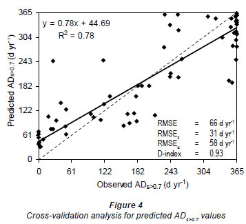
A cross-validation analysis (Fig. 4) indicated that Eq. (1) slightly overestimated lower AD_s>0.7 values and slightly underestimated higher AD_s>0.7 values. The overall agreement was very good, with a D-index of 0.93. The large unsystematic fraction of the total RMSE (RMSEu/RMSE = 0.88) indicated the absence of serious bias in model predictions. The model was therefore considered to be acceptable for predicting AD_s>0.7 values for soils in the Weatherley catchment.

 

 

There is an inherent hypothesis in the South African soil classification system (Soil Classification Working Group, 1991; Le Roux et al., 1999; Van Huyssteen and Ellis, 1997; Van Huyssteen et al., 1997) that diagnostic horizons contain integrated information about, inter alia, soil wetness. Equation (1) provides strong support for this hypothesis and therefore supports the use of soil classification for the prediction of duration of water saturation. This finding does, however, require further investigation and validation in other catchments.

 

Summary

Comparisons of the mean daily soil s values for the 0-900 mm layer (s_s) for different soils indicated general agreement with the pedologically expected wetness. The s_s values for the solum generally increased from the driest Tukulu, Avalon, and Hutton soils to the intermediate Bloemdal, Pinedene, and Longlands soils, and finally to the wettest Westleigh, Kroonstad, and Katspruit soils. The s_s values also generally increased downslope (from the crest to the valley bottom), and with decreasing slope and decreasing particle size. Significant correlations (α = 0.05) were obtained between s_s values and slope (R² = 0.24), coarse sand content (R² = 0.22), medium sand content (R² = 0.23), fine silt content (R² = 0.19), and clay content (R² = 0.38).

AD_s>0.7 values, averaged per diagnostic horizon type, ranged from 21 to 29 d•yr^-1 for the red apedal B, yellow brown apedal B, and neocutanic B; 103 d•yr^-1 for the orthic A horizons; and from 239 to 357 d•yr^-1 for the soft plinthic B, unspecified material with signs of wetness, E, and G horizons. Sand content, carbon to nitrogen ratio, and slope were negatively correlated with the mean daily s values for diagnostic horizons; while depth, clay to sand ratio, and base saturation were positively correlated.

A regression equation was developed to predict AD_s>0.7values from diagnostic horizon type (DH), clay to sand ratio (Cl:Sa), and underlying horizon type (DH ): AD_s>0.7 = -26.31 + 41.64 ln(Cl:Sa) + 35.43 DH + 13.73 DH_u (R² = 0.78). A model validation test gave an index of agreement of 0.93, a ratio of the unsystematic to the total root mean square error of 0.88, indicating that the results of the model were reliable. Diagnostic horizon was shown to have a strong influence on AD_s>0.7 emphasising the value of soil classification in the prediction of duration of water saturation.

 

Acknowledgements

Funding by the Water Research Commission, Mondi, North Eastern Cape Forests, the National Research Foundation, and the University of the Free State is gratefully acknowledged.

 

References

BEVEN KJ and KIRKBY MJ (1979) A physically based, variable contributing area model of basin hydrology Hydrol. Sci. Bull. 24 43-69.         [ Links ]

BEEH (2003) Weatherley Database V1.0. School of Bioresources Engineering and Environmental Hydrology, University of Natal, Pietermaritzburg.         [ Links ]

BLAVET D, MATHE E and LEPRUN JC (2000) Relations between soil colour and waterlogging duration in a representative hillside of the West African granito-gneissic bedrock. Geoderma 99 187-210.         [ Links ]

BURT TP and BUTCHER DP (1985) Topographic controls of soil moisture distributions. J. Soil Sci. 36 469-486.         [ Links ]

CANTON Y, SOLE-BENET A and DOMINGO F (2004) Temporal and spatial patterns of soil moisture in semi-arid badlands of SE Spain. J. Hydrol. 285 199-214.         [ Links ]

CODY RP and SMITH JK (1997) Applied Statistics and the SAS Programming Language (4th edn.). Prentice-Hall, New Jersey.         [ Links ]

DONKIN MJ and FEY MV (1991) Factor analysis of familiar properties of some Natal soils with the potential for afforestation. Geoderma 48 297-304.         [ Links ]

ESRI (1999) ArcView GIS V3.2. Environmental Systems Research Institute, Redlands, California.         [ Links ]

FAMIGLIETTI JS, RUDNICKI JW and RODELL M (1998) Variability in surface moisture content along a hillslope transect: Rattlesnake Hill, Texas. J. Hydrol. 210 259-281.         [ Links ]

FEKEDULEGN BD, COLBERT JJ, HICKS RR and SCHUCKERS ME (2002) Coping with multicollinearity: an example on application of principal components regression in dendroecology. Research paper NE-721. USDA Forest Service, Pennsylvania.         [ Links ]

GOMEZ-PLAZA A, MARTINEZ-MENA M, ALBALADEJO J and CASTILLO VM (2001) Factors regulating spatial distribution of water content in small semiarid catchments. J. Hydrol. 253 211-226.         [ Links ]

HE X, VEPRASKAS MJ, LINDBO DL and SKAGGS RW (2003) A method to predict soil saturation frequency and duration from soil color. Soil Sci. Soc. Am. J. 67 961-969.         [ Links ]

HENSLEY M and ANDERSON JJ (1998) Water Balance Studies at Four Locations at North East Cape Forests: 1998 Progress report to Mondi. ARC-Institute for Soil, Climate and Water, Pretoria.         [ Links ]

HILLEL D (1980) Applications of Soil Physics. Academic Press, New York.         [ Links ]

KUTILEK M and NIELSEN DR (1994) Soil Hydrology. Catena Verlag, Cremlingen-Destedt, Germany.         [ Links ]

LAND TYPE SURVEY STAFF (2000) Land types of South Africa. Mem. Agric. Nat. Resour. S. Afr. ARC-Institute for Soil, Climate and Water, Pretoria.         [ Links ]

LE ROUX PAL (1996) The Nature, Distribution and Genesis of Selected Redoximorphic Soils in South Africa [Afr. Die Aard, Verspreiding en Genese van Geselekteerde Redoksmorfe Gronde in Suid-Afrika]. Ph.D. Thesis. University of the Free State, Bloemfontein.         [ Links ]

LE ROUX PAL, ELLIS F, MERRYWEATHER FR, SCHOEMAN JL, SNYMAN K, VAN DEVENTER PW and VERSTER E (1999) Guidelines for the Mapping and Interpretation of Soils in South Africa. University of the Free State, Bloemfontein.         [ Links ]

LE ROUX PAL, HENSLEY M, DU PREEZ CC, KOTZE E, VAN HUYSSTEEN CW, COLLINS NB and ZERE TB (2005) The Weatherley Catchment: Soil Organic Matter and Vegetation Baseline Study. WRC Report No. KV 170/05. Water Research Commission, Pretoria.         [ Links ]

LIN HS, BOUMA,J, WILDING LP, RICHARDSON JL, KUTILEK M and NIELSEN DR (2005) Advances in hydropedology. Adv. Agron. 85 1-89.         [ Links ]

LIN HS, KOGELMANN W, WALKER C and BRUNS MA (2006) Soil moisture patterns in a forested catchment: A hydropedological perspective. Geoderma 131 345-368.         [ Links ]

MITASOVA H and HOFIERKA J (1993) Interpolation by regularized spline with tension: II. Application to terrain modelling and surface geometry analysis. Math. Geol. 25 657-669.         [ Links ]

MIYAZAKI T (1993) Water Flow in Soils. Marcel Dekker, New York.         [ Links ]

NCSS (1998) NCSS Help System: Multiple Regression. Kaysville, Utah.         [ Links ]

RABENHORST MC and PARIKH S (2000) Propensity of soils to develop redoximorphic color changes. Soil Sci. Soc. Am. J. 64 1904-1910.         [ Links ]

RABENHORST MC, BELL JC and MCDANIEL PA (1998) Quantifying soil hydromorphology. SSSA Spec. Publ. 54. SSSA, Madison, Wisconsin.         [ Links ]

SOIL CLASSIFICATION WORKING GROUP (1991) Soil classification - A taxonomic system for South Africa. Mem. Agric. Nat. Resour. S. Afr. No. 15. Department of Agricultural Development, Pretoria.         [ Links ]

TASSINARI C, LAGACHERIE P, BOUZIGUES R and LEGROS JP (2002) Estimating soil water saturation from morphological soil indicators in a pedologically contrasted Mediterranean region. Geoderma 108 225-235.         [ Links ]

VAN DER WATT HVH and VAN ROOYEN TH (1995) A Glossary of Soil Science (2nd edn.). Soil Sci. Soc. S. Afr., Pretoria.         [ Links ]

VAN HUYSSTEEN CW and ELLIS F (1997) The relationship between subsoil colour and degree of wetness in a suite of soils in the Grabouw district, Western Cape. I. Characterization of colour defined horizons. S. Afr. J. Plant & Soil 14 149-153.         [ Links ]

VAN HUYSSTEEN CW, ELLIS F and LAMBRECHTS JJN (1997) The relationship between subsoil colour and degree of wetness in a suite of soils in the Grabouw district, Western Cape. II. Predicting duration of water saturation of colour defined horizons. S. Afr. J. Plant Soil 14 154-157.         [ Links ]

VAN HUYSSTEEN CW, HENSLEY M, LE ROUX PAL, ZERE TB and DU PREEZ CC (2005) The Relationship between Soil Water Regime and Soil Profile Morphology in the Weatherley Catchment, an Afforestation Area in the North-Eastern Eastern Cape. WRC Report No K5/1317. Water Research Commission, Pretoria.         [ Links ]

VAN HUYSSTEEN CW, ZERE TB and HENSLEY M (2009a) Soil water variability in the Weatherley grassland catchment, South Africa: I. Evapotranspiration. S. Afr. J. Plant Soil 26 170-178.         [ Links ]

VAN HUYSSTEEN CW, ZERE TB and HENSLEY M (2009b) Soil water variability in the Weatherley grassland catchment, South Africa: II. Soil water content. S. Afr. J. Plant Soil 26 179-185.         [ Links ]

VEPRASKAS MJ, HE X, LINDBO DL and SKAGGS RW (2004) Calibrating hydric soil field indicators to long-term wetland hydrology. Soil Sci. Soc. Am. J. 68 1461-1469.         [ Links ]

WEBSTER R (1997) Regression and functional relations. Eur. J. Soil Sci. 48 557-566.         [ Links ]

WESTERN AW, GRAYSON RB, BLOSCHL G, WILLGOOSE GR and McMAHON TA (1999) Observed spatial organization of soil moisture and its relation to terrain indices. Water Resour. Res. 35 797-810.         [ Links ]

WILKS DS (1995) Statistical Methods in the Atmospheric Sciences: An Introduction. Academic Press, San Diego.         [ Links ]

WILLMOTT CJ (1981) On the validation of models. Physical Geogr. 2 184-194.         [ Links ]

 

 

Received 24 April 2009; accepted in revised form 5 October 2010.

 

 

* To whom all correspondence should be addressed. +2751 401 9247; fax: +2751 401 2212; e-mail: vhuystc@ufs.ac.za