


Serviços Personalizados
Artigo
 Inglês (pdf)
 Artigo em XML
 Referências do artigo
Indicadores

Links relacionados
-
 Citado por Google
 -
 Similares em Google
Compartilhar

 Permalink
Water SA
versão On-line ISSN 1816-7950
versão impressa ISSN 0378-4738
Water SA vol.36 no.1 Pretoria Jan. 2010
The link between Movability Number and Incipient Motion in river sediments
Neil ArmitageI,*; Albert RooseboomII
IDepartment of Civil Engineering, University of Cape Town, Private Bag X3, Rondebosch 7701, South Africa
IIDepartment of Civil Engineering, University of Stellenbosch, Private Bag X1, Matieland 7602, South Africa
ABSTRACT
The concept of incipient motion has been of continuing interest to researchers and engineers working with sediment movement in rivers. This paper takes a new look at the use of the Movability Number for the prediction of Incipient Motion – which is here defined in terms of Intensity of Motion. A relationship between Movability Number and Intensity of Motion is developed for flow with turbulent boundaries, using data from other researchers for Particle Reynolds numbers up to nearly 12 000. This allowed for a firmer definition of Incipient Motion as well as a new bedload transportation equation. Additional laboratory experimentation for Particle Reynolds number over the range 0.12-486 facilitated the improved prediction of Incipient Motion from a plot of the critical Movability Number vs. Particle Reynolds number for a wide range of boundary conditions from laminar to turbulent.
Keywords: Incipient Motion, Movability Number, river hydraulics, sediment transport.
List of symbols
| Bf | Width of a rectangular laboratory flume (mm) |
| d | Median sediment diameter (mm or m) |
| D | Hydraulic mean depth (m) |
| d/Y | Relative roughness |
| d% | Sediment diameter where % indicates the percentage of particles finer than the indicated value (mm) |
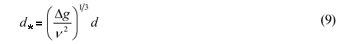
| d* | Dimensionless particle size |
| g | Gravitational acceleration (m·s-2) |
| I | Intensity of Motion (s-1) |
| m | Number of particle displacements during time t |
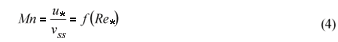
| Mn | Movability Number |
| Mnb | Flat bed Movability Number |
| Mnβ | Slope Movability Number |
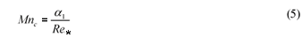
| Mnc | Critical Movability Number |
| N | Total number of surface particles over the sample area |
| qb | Sediment transport rate per unit width of bed (kg·m-1) |
 | Dimensionless bedload parameter |
| R2 | Correlation coefficient |
| Rb | Hydraulic radius associated with the bed zone (m) |
| Re* | Particle Reynolds number |
| s | Relative density |
| S0 | Bed slope |
| Sf | Friction slope |
| t | Time interval (t) |
| T | Temperature (ºC) |
| u* | Shear velocity (m·s-1) |
| u*/vss | Movability Number, Mn |
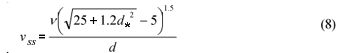
| vss | Settling velocity (m·s-1) |
| W* | Bedload parameter |
| Y | Depth of the flow (mm) |
| α1, α2 | Constants in the incipient motion equations |
| β | Longitudinal (streamwise) slope (degrees) |
| Δ | Relative submerged density |
| θ | Shields parameter |
| θc | Critical Shields parameter |
| ν | Kinematic viscosity of water (m2·s-1) |
| ρ | Density of water (kg·m-3) |
| ρs | Particle density (kg·m-3) |
| σgs | Graphic sorting coefficient |
| τ0 | Shear stress at the boundary (N·m-2) |
 r r | Angle of repose (degrees) |
| ξ | Exponent |
| ψ | Slope correction factor |
Introduction
The concept of incipient motion has been of continuing interest to researchers and engineers working with sediment movement in rivers. The fact that this seemingly simple concept still contains many mysteries is evident from the numerous publications that continue to appear in scientific journals to this day.
There are several ways of identifying the point of 'incipience', of which the best-known use parameters such as flow velocity, bed shear stress, or stream power. Most of the published literature uses the bed shear stress approach as popularised through the work of Shields (1936). A number of researchers, however, have preferred the use of the 'Movability Number' parameter introduced by Liu (1957). This parameter can be derived from considerations of velocity, bed shear stress or stream power (Armitage, 2002), and may thus provide a useful alternative to the better known Shields (1936) approach and its derivatives.
Key to the understanding of incipient motion is the definition of the rate of movement. Does the movement of a single grain on a riverbed constitute incipient motion of the bed? How about 1 grain per square metre of bed per second, and so forth? In other words, the incipient motion of a bed (as opposed to that of a grain) needs to be defined in terms of some 'Intensity of Motion'.
This paper takes a new look at the use of the Movability Number for the prediction of Incipient Motion – which is here defined in terms of a defined Intensity of Motion. Using data from other researchers for Particle Reynolds numbers up to nearly 12 000, a relationship between Movability Number and Intensity of Motion was developed for flow with turbulent boundaries. This allowed for a firmer definition of Incipient Motion as well as a new bedload transportation equation. Additional laboratory experimentation for Particle Reynolds number over the range 0.12 – 486 facilitated the prediction of Incipient Motion from a plot of the critical Movability Number vs. Particle Reynolds number for a wide range of boundary conditions from laminar to turbulent, which has extended the use of this approach.
Incipient Motion, intensity of motion and Movability Number
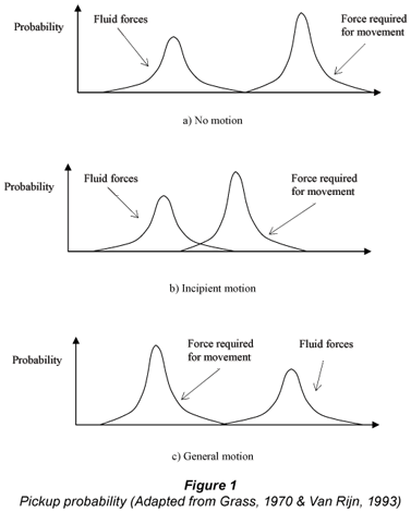
Incipient Motion, in the context of sediment transport in rivers, is that critical point at which sediment particles on the solid boundaries of the river flow (e.g. the bed or banks of a river) begin to move. From a theoretical point of view, if the fluid forces are below that required for the motion of a particle, there will not be any movement. If they are greater than that required for motion, there will be movement. The boundary between the two may be described as 'incipient' motion – i.e. the particle is about to move.
River beds are, however, comprised of millions of particles, each with a unique size, shape, electrical charge, density, packing and orientation, and subject to a unique instantaneous flow within the flow field. It is obvious that some particles are more easily moved than others; in other words, motion occurs with lower fluid forces than the average. On the other hand, the fluid forces also vary and an individual particle could be subjected to forces much higher than the average. Describing both the fluid forces required for incipient motion of individual particles, and the instantaneous fluid forces on any point of the boundary, in terms of probability density functions (e.g. Einstein, 1950; Grass, 1970; Van Rijn, 1993), and plotting them on the same axes, the probability of movement, or 'pickup probability', is associated with the overlap of the 2 probability density functions (Fig. 1).
Intensity of motion
Given the fact that neither probability density function has a clear cut-off value, there is always a statistical probability that a particle will move almost regardless of the flow conditions. At times, there appears to be little movement, whilst at other times there seems to be lots of movement. Given the stochastic nature of particle movement, it is probably more important to consider the rate at which particles are moved rather than talk of incipient motion. The motion might be of 1 or 2 particles only, several particles at a time, or involve general movement of the surface of the bed. Each level of movement is clearly associated with its own particular 'critical' conditions. This has been recognised by many researchers over the years, e.g. Kramer (1935), who defined 3 intensities of motion ('weak', 'medium' and 'general' movement) near the critical or threshold condition. More recently, Shvidchenko and Pender (2000a; b) defined I (s-1), the Intensity of Motion (or transport intensity), in terms of m, the number of particle displacements during the time interval t (s) and N, the total number of surface particles over the sample area, as:
They then defined 'weak sediment transport' as I = 10-4 s-1 (one of 10 000 surface particles is entrained every second), whilst 'general movement' was defined as I = 10-2 s-1 (one of 100 surface particles is entrained every second). Clearly it would be possible to define other transport rates should this be required. Another strategy is that which was adopted by Shields (1936), who attempted to find the critical shear stress for the initiation of movement by extrapolating a graph of observed sediment discharge versus shear stress to identify the value of apparent zero sediment discharge.
Movability Number
Some researchers have worked from the basis that the local flow velocity is the driving force behind sediment movement. One of the most prominent of these was Liu (1957) who came to the conclusion that the local velocity, and hence the various drag coefficients, were all functions of the Particle Reynolds number, Re*, defined as:
where:
d (m) is the particle diameter
v (m2·s-1) is the kinematic viscosity
u*(m·s-1) is the shear velocity defined as:
where:
τ0 (N·m-2) is the shear stress at the boundary
ρ (kg·m-3) is the fluid density
Liu then developed a new dimensionless parameter as the ratio of u* to the Particle Settling Velocity, vss (m·s-1) which he termed the 'Movability Number' and which will hereinafter be abbreviated to Mn. He came to the conclusion that for incipient motion there was a unique relationship between Mn and Re*, i.e.
The plot of the critical Mn value for incipient motion (Mnc) vs. Re* has a similar shape to the better known plot of the critical Shields parameter θc vs. Re* (the so-called 'Shields diagram'), with the advantage that sediment parameters such as diameter, shape factor and density – which help to make up θc – are effectively replaced by the single parameter of settling velocity. As with the Shields diagram, the plot does not include the flow velocity, local or average. Unlike the Shields diagram, however, there is no 'dip' of the curve in the transition zone (see, for example, Raudkivi, 1998) – making the plot slightly easier to use.
The basic form of the Mn – Re* plot can be predicted from unit stream power considerations. Rooseboom (1975) and Rooseboom and Le Grange (2000) showed that Mn can be understood in terms of the ratio of the applied unit stream power along the bed to the unit stream power required to keep the particles in suspension. Theoretically, for laminar boundary conditions:
whilst for turbulent boundaries:

In these 2 equations, a1 and a2 are empirical constants that were determined by Rooseboom (1975) from the then available data to be approximately equal to 1.6 and 0.12 respectively. The value of Re* also determines whether the boundary layer will be laminar, transitional or turbulent.
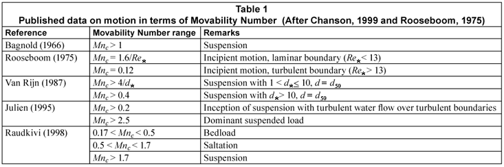
Other researchers have also noted relationships between Mnc and the intensity of motion. Considering only turbulent boundaries, Table 1 suggests that motion appears to commence once Mnc exceeds about 0.12, saltation commences once Mnc exceeds about 0.5, and suspension commences once Mnc exceeds about 1.0.
Turbulent boundary flow
Measurements of sediment transport over turbulent boundaries, made by 8 different researchers, were used to establish the link between Mn and I. The data were those used by Shvidchenko and Pender (2000a; b) in their work on incipient motion on flat beds (adopting the Shields, 1936 approach) and were kindly supplied to the principal author by the aforementioned researchers (Shvidchenko and Pender, 2001).
Data
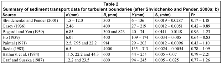
The data included both experimental measurements made by Shvidchenko and Pender (2001) as well as data collected by them from other sources. Correction was made for the influence of the sidewalls of the flumes using the method adopted by Shvidchenko and Pender (2000a; b). A summary of the data is presented in Table 2.
In Table 2, d (mm) is the median sand diameter, Bf (mm) is the width of the flume, Y (mm) is the depth, and S0 the bed slope. The sediment was gravel that could be considered reasonably uniform in each instance. Re* was high, averaging about 1 100 and never dropping below 36. The boundary flow conditions could thus be considered as completely turbulent over the entire data range. In all, there were 529 data points of which those obtained by Shvidchenko and Pender (2000a; b) made up 56% (297).
Conversion to Movability Number
The shear stress at the bed, τ0, was determined from:

where:
g (m·s-2) is gravitational acceleration
Rb (m) is the effective hydraulic radius operating on the bed after sidewall correction
S0 is the bed slope
This was then converted to u* with the aid of Eq. (3). The Cheng (1997) equation (Eq. (8)) was used to estimate the settling velocity, vss , of the sediment.
where:
d* is the dimensionless particle size given by Eq. (9):
where:
g (m·s-1) is the gravitational acceleration
d (m) is the sediment diameter)
ν (m2·s-1) is the kinematic viscosity for water
Δ is the relative submerged density given by Eq. (10):
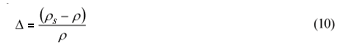
where:
ρs and ρ(both kg·m-3) are the sediment density and water density respectively
The kinematic viscosity for water, ν (m2·s-1) may be estimated by the Yang (1996) formulation:
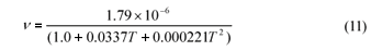
where:
T is the temperature (ºC).
Adjustment was also made for the bed slope. This was carried out with the aid of an equation adapted from Van Rijn (1993), and Chiew and Parker (1994):
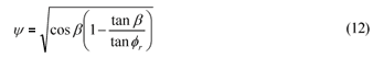
where:
β (degrees) is the longitudinal slope
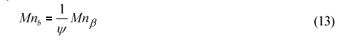
The effective flat bed Movability Number, Mnb, may then be determined from the slope Movability Number, Mnβ , via:
Estimation of the Intensity of Motion
Shvidchenko and Pender (2000a; b) not only counted the number of particle displacements during a given time interval, but also measured the sediment transport rate per unit width along the bed, qb (kg·m-1), associated with the Intensity of Motion. This was then expressed in terms of the dimensionless bedload parameter, , given by:
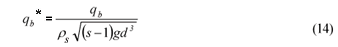
where:
s= the ρs/ρ the 'relative density'
The Shvidchenko and Pender (2000a; b) data showed that:

This equality allows any measured bedload transport rate to be expressed in terms of the intensity of sediment motion. In particular, it means that data collected by other researchers where the unit sediment transport rate had been measured could also be included in the data set for this exercise.
It should be noted that Eq. (15) is not dimensionally homogeneous (I has the units s-1 whilst is dimensionless). The Intensity of Motion, I, can, however, be understood as the probability that a particle in a bed area of length equal to the average length of displacement of a grain after detachment and unit width will start moving in any given second (Shvidchenko and Pender, 2000a).
Correction for relative roughness
At this point, an analysis of the complete data set showed that while there was a general relationship between I and Mn, there was also considerable scatter. In particular it was apparent that the Movability Number appeared to increase slightly with increasing bed-slope. Shvidchenko and Pender (2000a) had also noted that the critical bed shear stress (which is distantly related to Mn) appeared to increase with bed-slope. An increase in bed-slope (bearing in mind that a positive bed-slope is defined as a slope that falls in the direction of flow) should, however, lead to a decrease in the critical bed shear stress, and not vice versa. The reason for the discrepancy appeared to be the fact that all of the data come from experiments carried out in laboratory flumes. In consequence, the water depths in the various experiments all tend to decrease with increasing slope, giving rise to an increasing 'relative roughness' – sometimes to as much as d/Y = 0.5, where d is the median diameter of the particle and Y is the average depth. Correction had therefore to be made for relative roughness which was carried out as follows:
i) The following whole-number intensities of motion were selected: I = 10-2, 10-3, 10-4, 10-5, 10-6, 10-7, 10-8 s-1.
ii) Data with Intensity of Motion between 0.3 and 3 times a particular whole number selected from the list given in i) above was deemed to have that whole number Intensity of Motion. The values 0.3 and 3 were selected because they roughly represent the median point between 2 whole numbers on a logarithmic (Base 10) scale.
iii) The data associated with each intensity level was then plotted on a graph of Mn vs. relative roughness, d/Y (e.g. Fig. 2). A straight line, Eq. (12), was fitted through the data and extrapolated to zero relative roughness. A few high outliers (generally with d / Y > 0.3) were eliminated as they tended to distort the data.
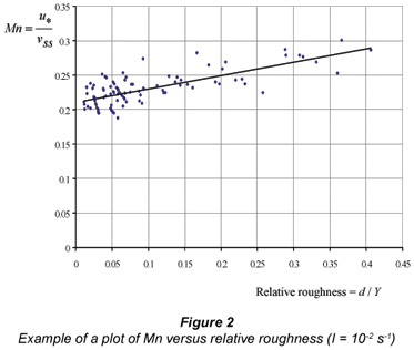
Once again, there was considerable scatter of the data, particularly with low intensities of motion. The mean gradient for the 4 highest intensities (I = 10-5 to 10-2 s-1) was 0.204. This represents the impact of relative roughness on the Mn associated with any particular I.
Movability Number vs. Intensity of Motion
A plot of the intercept values determined in iii) above vs. I gave the relationship between Mn and I for a flat bed with zero relative roughness (i.e. deep water). These values appeared to fall on a straight line with semi-logarithmic axes (Fig. 3).
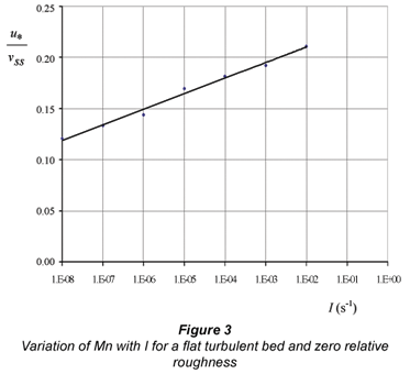
The equation of the line fitted to the data points (R2 = 0.9893) is:

The data were then adjusted for slope and relative roughness as follows:
The results of this adjustment are compared with the theoretical relationship in Fig. 4.
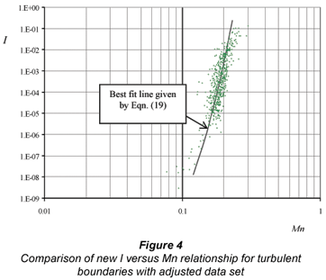
It will be noted from Fig. 4 that there is still considerable scatter – particularly at the low intensities of motion where there were few data, and accurate data were probably difficult to obtain.
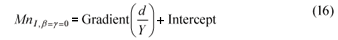
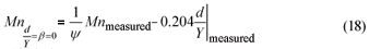
The final equation giving the relationship between Mn and I, taking into account the relative roughness, can now be written as follows:

New bedload transportation equation
The identity, I = (Eq. (15)) means that Eq. (19) may be rewritten:
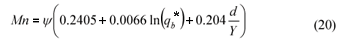
Rearrangement of Eq. (20) to makethe subject yields:

with the exponent, x, given by:
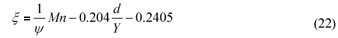
In Eq. (22), u* (for the calculation of Mn) may be estimated from Eq. (23):
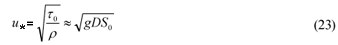
where:
D is the hydraulic mean depth
S0 is the bed slope
The settling velocity, vss, is best measured experimentally. Alternatively it may be estimated from the Cheng (1997) equation, Eq. (8). The unit bedload transport rate qb (kg·m-1), may then be determined from:

Experimental verification of Eq. (24) has not been carried out to date. Clearly its use is limited to situations where the flow boundaries are fully turbulent and little sediment is carried in suspension.
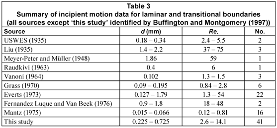
Laminar and transitional boundaries
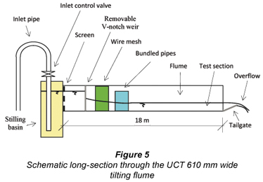
Buffington and Montgomery (1997) presented 613 measurements of critical shear stress values representing the collected work of numerous researchers over 8 decades (1914 – 1996). They included 56 measurements suitable for use in an analysis of the link between Mn and I for laminar and transitional boundaries. This data set was augmented by 41 experimental measurements made in the hydraulics laboratory at the University of Cape Town (UCT) – which were also corrected for the influence of the sidewalls (Fig. 5). The correction for the new experimental data was made using the so-called 'Einstein method' (Einstein, 1942; Chien and Wan, 1999), in conjunction with the Darcy-Weisbach equation, with the friction factor determined by the Barr (1975) approximation of the Colebrook-White equation (Colebrook and White, 1937; Colebrook, 1939), and adjusted for rectangular channels.
The following selection criteria were applied to the data sets:
• Only data involving the movement of natural quartzitic sand particles in water were used.
• The boundaries had to be laminar or transitional (loosely taken to be Re* < 75 although all except 4 values were under 30. (The higher values were useful to see how the transitional data linked with the turbulent data).
• The possible influence of sidewalls had to have been eliminated. This was achieved by a variety of methods. In some instances, the bed shear stress was determined from the velocity gradient. In other instances, correction factors were applied.
• The relative roughness had to be less than 5% (d/Y < 0.05) to ensure that this influence had been largely eliminated.
• The sediment had to be uniform. In the context of this study, this meant where sgs is the so-called graphic sorting coefficient (Buffington and Montgomery, 1997).
• As far as possible, the data were from plane beds. In practice this is very difficult to achieve as fine sediment (d < 0.7 mm) tends to form ripples immediately on onset of movement.
• In all cases incipient motion was determined through visual observation of the movement of the first few grains.
The data are summarised in Table 3. In all, 97 measurements satisfied the criteria.
For the laminar and transitional boundaries u* was calculated from:
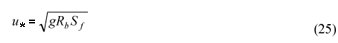
where:
Sf is the friction slope
New incipient motion criteria
The turbulent boundary data described previously covered a wide range of intensities of motion and relative roughness, d/Y. Shvidchenko and Pender (2000a; b) used I » 10-4·s-1 for their definition of incipient motion and compared it to the Kramer (1935) definition of 'weak' motion. Parker et al. (1982), meanwhile, introduced a bedload parameter, , and suggested a value of W* = 0.002 as a reference transport rate corresponding to threshold conditions. According to Shvidchenko and Pender (2000a), this corresponds to I » 3 x 10⁻⁵·s-1. Numerical modelling undertaken at UCT as part of this investigation (McGahey and Armitage, 2001; Armitage, 2002) appeared to give the best results with I = 2 x 10⁻⁵·s-1. A decision was thus made to examine the turbulent boundary data in the region of 3 x 10⁻⁶·s-1 < I < 3 x 10⁻⁴·s-1. In an attempt to reduce the impact of relative roughness without resorting to the use of empirical equations, the data set was further reduced to include only those values for which d/Y < 0.05 (as for the laminar and transitional boundary data). This reduced the turbulent boundary data set to 35 values, taken from 5 investigators (Table 4).

These data were added to those for laminar and transitional boundaries (Table 3) to give 132 values indicating the visual commencement ('weak') movement of natural uniform quartzitic sand on a flat bed with low relative roughness. The data were collected by 15 different researchers or groups of researchers, and covered the range of Re* from 0.12 to 486. They were then plotted on a graph of Mn vs. Re* (Fig. 6). For convenience, the turbulent boundary data for the 4 researchers, excluding Shvidchenko and Pender (2001), has been labelled 'Other turbulent boundary data' in Fig. 6.
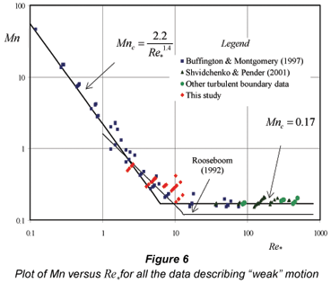
As could be expected, the data may be roughly grouped into 3 categories, that measured on laminar boundaries (Re*< 5), that measured on transitional boundaries (5 < Re*< 75), and that measured on turbulent boundaries (Re* > 75). A line corresponding to Mn = 0.17 seemed to fit the turbulent boundary data quite well, i.e. α2 = 0.17 in Eq. (6). In the case of the laminar boundary data, however, Mn appeared to vary with Re*-1.4 rather than Re*-1 as suggested by Eq. (5). The 2 new incipient motion equations (plotted in Figs. 6 and 7) marking the division between scour and deposition are thus:
The transitional boundary data seem to smoothly link these two equations. If these are ignored, the 2 curves join at Re* = 6.23. For comparison, the Rooseboom (1975) curves (Eqs. (5) and (6)) are also plotted on Fig. 6. It is not certain why the laminar boundary data do not behave as predicted by Eq. (5). Perhaps it is because of increasing inter-particle cohesion with decreasing particle size.
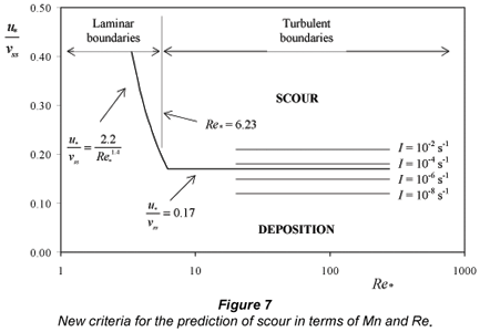
It must be emphasised that whilst Eqs. (26) and (27) summarise the data quite well, they only indicate the point at which there is noticeable movement of particles along the bed. Figure 7 is a plot of Mn vs. Re*, showing both the lines indicated by Eqs. (26) and (27) for incipient motion as defined, and, for turbulent boundaries only, the significance of different intensities of motion, I. There were insufficient data to determine I for laminar and transitional boundaries.
Conclusions
The subject of this paper was the determination of alternative criteria for incipient motion using the Movability Number, Mn, as defined by Liu (1957). The main problem was that sediment motion could theoretically occur in any flow state. The solution to this was to define Incipient Motion in terms of a specified Intensity of Motion, I (Shvidchenko and Pender, 2000a; b).
Data supplied by Shvidchenko and Pender (2001) for turbulent boundaries were processed into a new equation linking Mn with I, taking into account the bed-slope and relative roughness. This was readily transformed into a new bedload transportation equation.
Additional data gathered for flow with laminar and transitional boundaries were combined with the data for turbulent boundaries and used to develop new Incipient Motion criteria for a flat bed comprising uniform cohesionless quartzitic particles (Eqs. (26) and (27) or Figs. 6 and 7). In the instance of turbulent beds, the criterion for visual observation of the movement of the first few grains equates to an Intensity of Motion, I, of 2 x 10⁻⁵. Adjustment may be made for other values of I if so wished.
The linking of Mn with I over a wide range of particle Reynolds numbers and the subsequent development of a new bedload transportation equation represent an original contribution to the debate on incipient motion.
Acknowledgements
The information contained in this paper was funded by the Water Research Commission of South Africa under WRC Project No. K5/1098: 'An investigation into the critical conditions for the deposition and re-entrainment of natural sediments and litter in the rapidly varied open channel flow through hydraulic structures' and published as WRC Report No. 1098/1/03 entitled: A Unit Stream Power Model for the Prediction of Local Scour in Rivers (Armitage and McGahey, 2003).
References
ARMITAGE NP (2002) A Unit Stream Power Model for the Prediction of Local Scour. Unpublished Ph.D. Dissertation, University of Stellenbosch, Stellenbosch, South Africa. [ Links ]
ARMITAGE N and MCGAHEY C (2003) A Unit Stream Power Model for the Prediction of Local Scour in Rivers. WRC Report No. 1098/1/03, Water Research Commission, Pretoria, South Africa. [ Links ]
BAGNOLD RA (1966) An approach to the sediment transport problem from general physics. US Geol. Surv. Prof. Paper 422-I. 37 pp. [ Links ]
BATHURST JC, CAO HH and GRAF WH (1984) Hydraulics and Sediment Transport in a Steep Flume: Data from the EPFL Study. Report of the Institute of Hydrology, Wallingford. [ Links ]
BARR DIH (1975) Two additional methods of direct solution of the Colebrook-White function. Proc. Inst. Civ. Eng. Part 2 59 827-835. [ Links ]
BOGARDI J and YEN CH (1939) Traction of Pebbles by Flowing Water. Ph.D. Dissertation, State University of Iowa, USA (as cited in: Brownlie WR (1981) Compilation of Alluvial Channel Data: Laboratory and Field. W.M. Keck Laboratory of Hydraulics and Water Resources, California Institute of Technology, Pasadena, California. Report No. KH-R-43B). [ Links ]
BUFFINGTON JM and MONTGOMERY DR (1997) A systematic analysis of eight decades of incipient motion studies, with special reference to gravel-bedded rivers. Water Resour. Res. 33 (8) 1993-2029. [ Links ]
CASEY HJ (1936) Über Geschiebebewegung. Mitteilungen der Preussischen Versuchsanstalt für Wasserbau und Schiffbau (Berlin) 19 86. [ Links ]
CHANSON H (1999) The Hydraulics of Open Channel Flow. Edward Arnold, London, UK. CHENG N-S (1997) Simplified Settling Velocity Formula for Sediment Particle. J. Hydraul. Eng. ASCE 123 (2) 149-152. [ Links ]
CHIEN N and WAN Z (1999) Mechanics of Sediment Transport. ASCE Press, New York, USA. [ Links ]
CHIEW Y-M and PARKER G (1994) Incipient sediment motion on non-horizontal slopes. J. Hydraul. Res. 32 (5) 649-660. [ Links ]
COLEBROOK CF and WHITE CM (1937) Experiments with fluid friction in roughened pipes. Proc. R. Soc. London A161 367-381. [ Links ]
COLEBROOK CF (1939) Turbulent flows in pipes, with particular reference to the transition region between the smooth and rough pipe laws. J. Inst. Civ. Eng. 11 133-156. [ Links ]
EINSTEIN HA (1942) Formulas for the transportation of bed load. Trans. ASCE 107 575-577. [ Links ]
EINSTEIN HA (1950) The Bed Load Function for Sediment Transportation in Open Channel Flows. Technical Bulletin 1026. U.S. Department of Agriculture, Washington, DC. [ Links ]
EVERTS CH (1973) Particle overpassing on flat granular boundaries. J. Hydraul. Div. ASCE 99 425-439. [ Links ]
FERNANDEZ LUQUE R and VAN BEEK R (1976) Erosion and transport of bedload sediment. J. Hydraul Res. 14 127-144. [ Links ]
GRAF WH and SUSZKA L (1987) Sediment transport in steep channels. J. Hydrosci. Hydraul. Eng. (Japan Society of Civil Engineers) 5 (1) 11-26. [ Links ]
GRASS AJ (1970) Initial instability of fine bed sand. J. Hydraul. Div. ASCE 96 (HY3) 619-632. [ Links ]
HO P-Y (1939) Abhangigkeit der Geschiebebewegung von der Kornform und der Temperature. Mitteilungen der Preussischen Versuchsanstalt für Wasserbau und Schiffbau (Berlin) 39 43. [ Links ]
IKEDA H (1983) Experiments on Bedload Transport, Bed Forms, and Sedimentary Structures Using Fine Gravel in the 4-meter-wide Flume. Report of the Environmental Research Center, University of Tsukuba, No. 2, Tokyo. [ Links ]
JULIEN PY (1995) Erosion and Sedimentation. Cambridge University Press, Cambridge, UK. 280 pp. [ Links ]
KRAMER H (1935) Sand mixture and sand movement in fluvial model. Trans. ASCE 100 798-873. [ Links ]
LIU H-K (1957) Mechanics of sediment-ripple formation. J. Hydraul. Div. ASCE 83 (HY2) 23 pp. [ Links ]
LIU T-Y (1935) Transportation of the Bottom Load in an Open Channel. M.Sc. Thesis, University of Iowa, Iowa City, USA. 34 pp. [ Links ]
MANTZ PA (1975) Low Transport Stages by Water Streams of Fine, Cohesionless Granular and Flaky Sediments. Ph.D. dissertation, University of London, London. [ Links ]
McGAHEY C and ARMITAGE NP (2001). A three-dimensional numerical model for scour prediction based on the unit stream power approach. Proc. 10th S. Afr. Natl. Hydrol. Symp. Pietermaritzburg, South Africa. 11 pp. [ Links ]
MEYER-PETER E and MULLER R (1948). Formulas for bed-load transport. Proc. 2nd Meeting of the International Association for Hydraulic Structures Research. IAHR, Delft, Netherlands. 39-64. [ Links ]
PAINTAL AS (1971) Concept of critical shear stress in loose boundary open channels. J. Hydraul. Res. 9 91-113. [ Links ]
PARKER G, KLINGEMAN PC and McLEAN DG (1982) Bedload and size distribution in paved gravel-bed streams. J. Hydraul. Div. ASCE 108 544-571. [ Links ]
RAUDKIVI AJ (1963) Study of sediment ripple formation. J. Hydraul. Div. ASCE 89 15-33. [ Links ]
RAUDKIVI AJ (1998) Loose Boundary Hydraulics. A. A. Balkema, Rotterdam. [ Links ]
ROOSEBOOM A (1975) Sediment Transport in Rivers and Reservoirs. D.Eng. Dissertation, University of Pretoria, South Africa (in Afrikaans). [ Links ]
ROOSEBOOM A and LE GRANGE A (2000) The hydraulic resistance of sand streambeds under steady flow conditions. J. Hydraul. Res. 38 (1) 27-35. [ Links ]
SHIELDS A (1936) Anwendung der Aenlichkeitsmechanik und der Turbulenzforschung auf die Geschiebebewegung. Mitteilungen der Preussischen Versuchsanstalt für Wasserbau und Schiffbau No. 6, Berlin, Germany (in German). (English translation by WP Ott and JC van Uchelen, Hydrodynamics Laboratory Publication No. 167, Hydrodynamics Lab. California Inst. of Technology, Pasadena, USA). [ Links ]
SHVIDCHENKO AB and PENDER G (2000a) Flume study of the effect of relative depth on the incipient motion of coarse uniform sediments. Water Resour. Res. 36 (2) 619-628. [ Links ]
SHVIDCHENKO AB and PENDER G (2000b) Initial motion of streambeds composed of coarse uniform sediments. Proc. Inst. Civ. Eng. Water Mar. Eng. 142 (Dec.) 217-227. [ Links ]
SHVIDCHENKO AB and PENDER G (2001) Personal communication with Andrey Shvidchenko and Gareth Pender, School of the Built Environment, Heriot Watt University, Edinburgh, Scotland, UK. [ Links ]
USWES (1935) Study of river-bed material and their use with special reference to the Lower Mississippi River. Paper 17, US Waterways Experimental Station, Vicksburg, Mississippi, 161 pp. [ Links ]
VAN RIJN LC (1987) Mathematical Modeling of Morphological Processes in the Case of Suspended Sediment Transport. Ph.D. Thesis, Delft University of Technology, Delft, The Netherlands. [ Links ]
VAN RIJN LC (1993) Principles of Sediment Transport in Rivers, Estuaries and Coastal Seas. Aqua Publications, Blokzijl, The Netherlands. [ Links ]
VANONI VA (1964) Measurements of Critical Shear Stress for Entraining Fine Sediments in a Boundary Layer. KH-R-7, W. M. Keck Lab., Hydraul. Water Res. Div. Eng. Appl. Sci., Calif. Inst. of Technol., Pasadena. 47 pp. [ Links ]
YANG CT (1996) Sediment Transport: Theory and Practice. McGraw-Hill, New York, USA. [ Links ]
Received 5 June 2009; accepted in revised form 12 November 2009.
* To whom all correspondence should be addressed.
+2721 650 2589; fax: +2721 689 7471;
e-mail: Neil.Armitage@uct.ac.za

