Conveyance estimation in channels with emergent bank vegetation

 

 

PM Hirschowitz^*; CS James

Centre for Water in the Environment, School of Civil & Environmental Engineering, University of the Witwatersrand, Private Bag 3, Wits, 2050, South Africa

 

 

---

ABSTRACT

Emergent vegetation along the banks of a river channel influences its conveyance considerably. The total channel discharge can be estimated as the sum of the discharges of the vegetated and clear channel zones calculated separately. The vegetated zone discharge is often negligible, but can be estimated using established methods if necessary. The clear channel discharge can be estimated either through application of a resistance equation using a composite resistance coefficient, or by integration of the transverse distribution of the depth-averaged velocity. Recommendations are made for estimating the composite resistance coefficient, and the coefficient for the vegetation interface. An equation for the integrated velocity distribution is also presented, together with a procedure for its application. The methods reliably reproduce resistance coefficients and conveyances measured in laboratory channels

Keywords: flow resistance, bank vegetation, vegetated channels

---

 

 

Nomenclature

A	cross-sectional area
ax	longitudinal spacing of vegetation stems
B	clear channel bed width
bm	transition width within vegetation
bf	transition width within vegetation plus half or full clear channel width
bfo	half or full clear channel width
CD	vegetation stem drag coefficient
D	flow depth
d	vegetation stem diameter
F	resistance coefficient for vegetation
f	Darcy-Weisbach resistance coefficient
fb	resistance coefficient for bed
fI	flow interaction contribution to fv
fTo	vegetation structure contribution fv
fv	resistance coefficient for vegetation interface
g	gravitational acceleration
hT	flow depth at vegetation interface
K	empirical constant equal to 2.2
l	concentration length for flow through vegetation
n	Manning' s resistance coefficient
Q	discharge
R	hydraulic radius
Rv	vegetation zone hydraulic radius
S	channel energy slope
s	vegetation stem spacing
T	transition width in clear channel
Twide	transition width for narrow clear channel
Tnarrow	transition width for wide clear channel
u*v	shear velocity on vegetation interface
V	depth-averaged velocity
Vinf	depth-averaged velocity unaffected by vegetation
V/max	dimensionless maximum velocity
Vmax	maximum depth-averaged velocity on transverse profile
Vveg	velocity within vegetated zone
y	transverse distance measured from an origin within the vegetation
ρ	water density
τ	shear stress on bed

 

Introduction

Vegetation, (for example reeds) occurs commonly along the banks and instream bars of rivers, and is often emergent during low flows. Emergent bank vegetation has significant influence on the channel hydraulics, including the turbulence structure (e.g. Choi and Kang, 2006 and Nadaoka and Yagi, 1998), velocity distribution (e.g. Nuding, 1991; 1994), and the overall conveyance (e.g. James et al., 2001). Depending on the application required, these phenomena and their effects can be described at different levels of resolution. Many environmental and engineering applications require only prediction of flow depths and cross-section average velocities for specified discharges, however, which do not usually require high resolution modelling. This paper focuses on the relation between discharge and flow depth at low flows, and is intended to contribute primarily to environmental studies. As such, it considers only the hydraulic influence of in-channel bank vegetation where the water surface is below both the top of the vegetation (i.e. the vegetation is emergent) and the top of the banks. The hydraulics of this situation differs from that of floodplain vegetation in a compound channel (Helmiö, 2004), and the methods proposed cannot be applied to overbank flows. In view of the limited data generally available for environmental studies, the methods described are simple enough to be used with limited site data.

 

Vegetated zone discharge

Following the flow-resistance approach, the discharge in a channel zone can be calculated from the gross continuity formulation:

where:

Q is the appropriate zonal discharge
A is the corresponding zonal cross-sectional flow area
V is the average velocity over this area

The flow contribution of vegetated zones is usually relatively small and can be ignored in many situations. Where it is significant, it can be estimated using methods proposed for flow through emergent vegetation, such as from Eq. (1) (James et al., 2008) with the velocity within the vegetation given by:

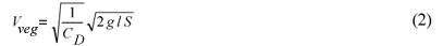
where:

where:

s is the average clear stem spacing
S is the channel energy slope
d is the stem diameter
g is gravitational acceleration
C_D is the stem drag coefficient (James et al., 2008)

A modified form of Eq. (2) including a term for the substrate resistance is provided by James et al. (2008) for sparse vegetation where the substrate resistance is significant. Values of C_D can be estimated as described by James et al. (2008) and Jordanova et al. (2006). If appropriate field data are available, it is preferable to calibrate directly an alternative form of Eq. (2) (James et al., 2004) with variables lumped as:

where:

F is a site-specific resistance coefficient (James et al., 2004)

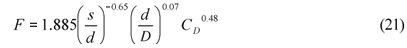
An empirical equation for the lumped resistance F for reeds, derived by Jordanova et al. (2006), is used here, and is presented as Eq. (21) below.

 

Clear channel discharge from resistance calculations

The discharge in the clear, un-vegetated zone between the bank vegetation strips can be calculated from Eq. (1) with V calculated by a conventional resistance equation. Here the Darcy-Weisbach equation is used, i.e.:

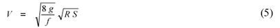
where:

g is gravitational acceleration
f is the effective resistance coefficient
R is the hydraulic radius
S is the friction slope (equal to the channel slope for steady, uniform flow)

In Eq. (5), f is a composite friction factor accounting for resistance by the bed and the interfaces between the vegetated and un-vegetated zones. An expression for f in terms of the contributing surface values can be obtained by balancing the stream-wise weight component of steady, uniform flow with the resisting shear forces on the bed and interfaces. The boundary shear stresses can be expressed in terms of the corresponding resistance coefficients as:

where:

τ is shear stress and
ρ is the water density

For a clear channel width B with vegetation on both sides, the force balance then leads to:

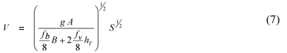
where:

A is the cross-section area of the un-vegetated zone
B is the bed width
h_T is the flow depth at the interface
f_b is the friction factor of the bed
f_v is the friction factor of the vegetation interface

Combining this with Eq. (5) yields the composite resistance coefficient:

which is equivalent to the composite roughness formula proposed by Pavlovski (1931) for different roughnesses on a horizontal bed in terms of Manning's n

Note that for other arrangements, Eqs. (7) and (8) would be modified to reflect the actual boundaries of the non-vegetated zone. For example, in the case of vegetation on one side and a solid boundary on the other side, 2f_v would be replaced by f_v+f_side where f_side is the resistance coefficient of the solid boundary

James and Makoa (2006) confirmed the reliability of Eqs. (1), (5) and (8) for predicting clear channel discharges in laboratory and field situations, but provided no guidance for estimating f_v. This coefficient represents the momentum absorbing capacity of the vegetation zone and depends on the vegetation characteristics within the zone as well as the flow conditions in the clear channel. Methods for estimating f_v have been reviewed by Hirschowitz (2006), and include those proposed by Pasche and Rouvé (1985), Bertrams (1985), Mertens (1989), Kaiser (1984) and Nuding (1991, 1994). The method of Pasche and Rouvé (1985) was developed for vegetation in compound channels and is not usable where the vegetation is not on an elevated flood plain. The method of Bertrams (1985) was found to give unrealistic predictions, while its extension by Mertens (1989) includes an unknown empirical coefficient. The methods of Kaiser (1984) and Nuding (1991; 1994) are therefore candidates for practical applications and have been tested against independent laboratory measurements

According to Kaiser (1984) the value of f_v is given by:

where:

f_τo is due to the vegetation structure and has a value between 0.06 and 0.10
f_I is due to the flow interaction

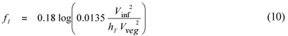
where:

V_inf is the depth-averaged velocity that would occur as a result of bed resistance only without the influence of vegetation
V_veg is the unaffected velocity within the vegetation
h_T is measured in metres (the number 0.0135 is also a length in m).

Nuding (1991, 1994) gives the interface friction factor as:

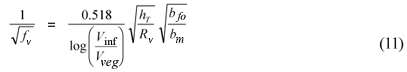
where:

R_v is the hydraulic radius of the vegetated zone
b_fo is half the width of the clear channel if it is bounded by vegetation on both sides and the full clear channel width if it is bounded by vegetation on one side and a surface offering negligible resistance on the other

The distance b_m is a transition width within the vegetation, given by the smallest of the following:

• Lateral spacing of the vegetation stems
• Wake width, given by 3.2(a_x.d)^1/2, where a_x is the longitudinal spacing of vegetation stems and d is the stem diameter
• Actual width of the vegetation strip

Additionally, b_m may not be less than 0.15h_T

 

Clear channel discharge from integrated velocity distribution

The clear channel discharge can also be predicted by integrating the transverse distribution of depth-averaged velocity. Hirschowitz and James (2008) have reviewed and tested various equations proposed for describing the transverse distribution of depth-averaged longitudinal velocity in clear channel flow adjacent to emergent vegetation boundaries. They recommend a refinement of the method proposed by Nuding (1991; 1994), with the velocity at position y given by the lesser of:

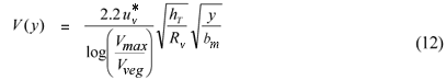
or

where:

y is measured from an origin at distance b_m from the vegetation interface within the vegetation
u_v^* is the shear velocity on the vegetation interface
V_veg is the velocity within the vegetation (which may be calculated from Eqs. (2) and (3) or (4))
V_max is the maximum velocity within the clear channel zone

The maximum velocity in the clear channel is calculated using a dimensionless maximum velocity:

where:

V_inf is the velocity that would occur in the channel under the resistance influence of the bed only

The dimensionless maximum velocity is calculated from an empirically-derived equation:

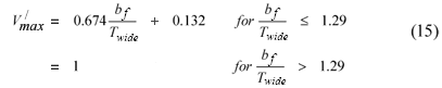
where:

b_f is the value of y at the channel centre for channels with vegetation on both sides or at the non-vegetated bank for channels with vegetation on one side only
T_wide is the width over which the transition from V_veg to V_max takes place in a channel that is wide enough for V_max = V_inf.
T_wide is given by:

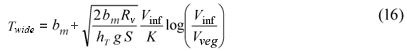
The value of u_v^* depends on whether the clear channel zone is wide or narrow, i.e. is b_f greater or less than 1.29T_wide. For the wide case u_v^* can be calculated directly as:

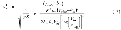
For narrow clear channel zones u_v^* must be determined iteratively. A transition width, T_narrow is estimated and used as the value for b_f in calculating u_v^* according to:

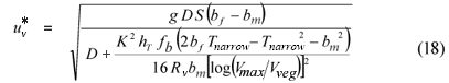
where:

D is the flow depth

Using this result, T_narrow is calculated as:

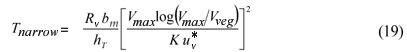
Equations (18) and (19) are applied iteratively until satisfactory convergence of the T_narrow and u_v^* values

The relevant values of V_max and u_v^* enable the description of the velocity profile through Eqs. (12) and (13), which can be integrated across the clear channel width to yield the clear channel zone discharge (Hirschowitz, 2006):

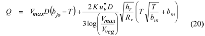
where:

T is the appropriate transition width depending on whether the zone is wide or narrow

 

Experimental data

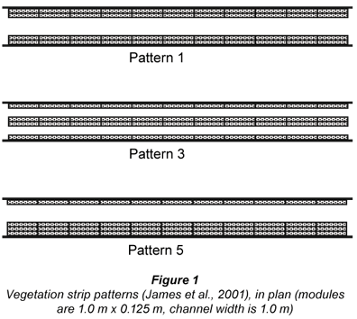
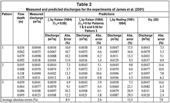
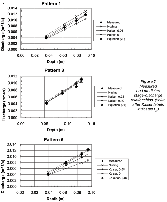
Suitable data for testing these prediction methods were collected by James et al. (2001) and James and Makoa (2006). Their experiments were carried out in a 12.26 m long, 1.0 m wide, rectangular channel lined with cement plaster and set on a slope of 0.00107. Vegetation stems were represented by 5 mm diameter steel rods set in a regular, staggered grid pattern with centre spacings of 25 mm in both the longitudinal and transverse directions. The rods were secured above the water surface in wooden frames, each 1.0 m long and 0.125 m wide and holding 200 rods, enabling their arrangement in 7 distribution patterns, of which the 3 shown in Fig. 1 are useful for testing predictions. All the patterns extended over a distance of 11.0 m and contained the same total number of stems, with the same local density and the same overall coverage (50% of the channel area). Stage-discharge measurements were taken for all patterns and for the basic channel with no stems. Longitudinal velocities were measured over one cross section of each clear channel using a miniature propeller meter. Velocities were measured at a number of vertical sections, with spacing depending on the clear channel width, and at 0.2, 0.4 and 0.8 of the flow depth.

 

 

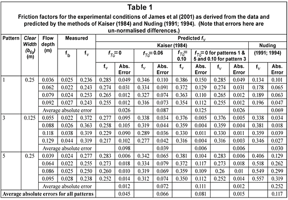
The resistance coefficient for the bed (f_b) was determined as a function of flow depth from measured stage-discharge data for the basic channel with no artificial vegetation. The data presented by James et al. (2001) included 9 combinations of depth and discharge for the basic channel, with depths ranging from 21 mm to 72 mm. f_b was calculated for each of these tests through Eqs. (1) and (5). A quadratic equation for f_b in terms of flow depth was fitted through these points, and used to determine f_b for each vegetated channel depth. The resulting values of f_b ranged from 0.022 to 0.044 with 10 of the 12 values occurring between 0.022 and 0.028. Resistance coefficients for the bed and the stem zone interfaces (f_v) were also determined for Patterns 1, 3 and 5, through an inverse application of the sidewall correction procedure proposed by Brownlie (1981). The values determined are listed in Table 1.

 

 

Applications

The methods of Kaiser (1984) and Nuding (1991; 1994) have been applied to the experimental situations to predict values of f_v. The results are presented in Table 1 and Fig. 2. For the method of Kaiser (1984), values of f_To of 0.06 (the minimum value recommended by Kaiser , 1984) and 0.10 (the maximum value recommended by Kaiser, 1984) are both presented. Both methods perform satisfactorily for the narrow clear channel of Pattern 3: average absolute errors (the absolute difference between predicted and measured values) are 0.030 for Nuding's method and 0.039 and 0.006 for Kaiser's method with f_To equal to 0.06 and 0.10 respectively. Performance is less satisfactory for Patterns 1 and 5 with relatively wide clear channels. For

 

 

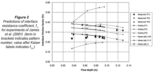
Pattern 1, average absolute errors are 0.069 for the method of Nuding (1991; 1994), 0.087 for the method of Kaiser (1984) with f_t0 = 0.06 and 0.125 f_t0 = 0.1. Similarly, large prediction errors are also found for Pattern 5 as indicated in Table 1.

While the data suggest that clear channel width is influential, neither method accounts for it satisfactorily. The method of Nuding (1991; 1994) accounts for width explicitly through the inclusion of b_fo in Eq. (11), but does not reproduce the trend of f_v with D well for either the narrow or wide channels (Fig. 2). The extreme difference in predictions for Patterns 1 and 5 arises from the definition of b_m, giving significantly different values for these 2 patterns, even though the clear channel width is the same. The method is therefore unrealistically sensitive to this definition, and hence to the width of vegetation strips which appears to be influential only at very low flow depths. Kaiser's (1984) method reproduces the trend of f_v with D well for both the narrow and wide clear channels (Fig. 2). The position of the curves depends only on the value selected for f_To but, perhaps coincidentally, could account for clear channel width. Although Kaiser intended f_To to account for vegetation structure, it is not unreasonable to suppose that this effect becomes less important relative to the ratio V_inf/V_veg as channel width increases

Setting f_To = 0 (i.e. neglecting the vegetation structure term) leads to very close agreement of Kaiser's (1984) method with the data for the wide clear channels, with an absolute average error for Patterns 1 and 5 of only 0.026 and 0.012 respectively, and with just 2 points giving errors greater than 0.018 (See Table 1). However, the prediction accuracy for pattern 3 with a narrow clear channel is reduced from that obtained with f_To = 0.1. The best prediction (average absolute error of 0.015 for all three patterns) is thus given by selecting f_To = 0 for wide clear channels (patterns 1 and 5) and f_To = 0.1 for narrower clear channels (pattern 3). This confirms that the vegetation structure term (f_To) is effective only for narrow channels. As the width to depth ratios (B/D) occurring in Patterns 1 and 5 are more representative of real channels than those of Pattern 3, Kaiser's method with f_To = 0 appears to be the best currently available for estimating the f_v for emergent vegetation lateral boundaries.

The velocity measurements were integrated to obtain clear channel discharges for the three vegetation patterns. These were also predicted using Eqs. (1), (5) and (8) with f_v estimated by the methods of Kaiser (1984) and Nuding (1991; 1994). Kaiser's (1984) method was applied with f_To = 0.08 (the middle value of the recommeded range) and also with f_To = 0.1 (the maximum value recommended) for conditions with B/D < 5 (Pattern 3) and f_To = 0 for B/D > 5 (Patterns 1 and 5) as described above. In these predictions V_inf was estimated using Eq. (5) with R equal to D and f_b was estimated as a function of depth (D) using results of experiments in the basic channel with no stems, as described above. The value of V_veg was determined using the method proposed by Jordanova et al. (2006), i.e. Eq. (4) with:

The stage-discharge predictions by the methods of Kaiser (1984) and Nuding (1991; 1994) as well as the integrated transverse velocity distribution (Eq. (20)) are compared with the measured data in Table 2 and Fig. 3. Discharge predictions by all methods are acceptable. Overall, Kaiser's (1984) method with f_To selected on the basis of B/D performs best, with an average absolute error of 2.6%. Equation (20), with an average absolute error of 7.0%, performs better than both Kaiser's (1984) method as originally intended and Nuding's (1991, 1994) method, with average absolute errors of 8.9% and 13.5% respectively. Equation (20) relies on the assumption of a constant depth and roughness within the clear channel, which may not be realistic in some real channels. The resistance equation approaches are more flexible, and could account for variations in channel characteristics. Of these, the method of Kaiser (1984) appears to be better than Nuding's (1991; 1994) even without adjusting f_To. Assigning a value of f_To = 0 for wide natural channels appears to be appropriate, but this is rather arbitrary and requires confirmation with appropriate data.

 

 

 

 

Conclusions

The conveyance of river channels with emergent vegetation along their banks can be estimated by adding discharges calculated separately for vegetated zones and clear channel zones. The contribution from the vegetated zones is often negligible, but may be estimated by existing methods (e.g. James et al., 2008 and Jordanova et al., 2006). The conveyance of the clear channel zones can be estimated through composite resistance calculations or by an integration of the transverse distribution of depth-averaged velocity.

For resistance calculations a composite resistance coefficient combining the effects of the channel bed and vegetation interfaces is used, as given by Eq. (8). The vegetation interface resistance coefficient (f_v) is best estimated by the method of Kaiser (1984) (Eqs. (9) and (10)). There are indications that f_To in Eq. (9) may depend on the width of the clear zone. A value of f_To = 0 appears to be appropriate for clear channels with B/D > ~5 while the range of 0.06 ≤ f_To<≤ 0.1 (as originally suggested by Kaiser, 1984) may be appropriate for narrower channels.

The transverse velocity distribution across the clear channel zone reflects the resisting influence of the boundaries, and its integration (Eq. (20)) to estimate conveyance would be particularly useful in cases where the velocity distribution is required as well. The implied assumption of constant depth and bed roughness within the clear channel may lead to inaccuracies in some natural channels, however, and the simpler composite resistance approach may be generally preferable.

 

Acknowledgements

This material is based upon work supported by the National Research Foundation (South Africa) and the Water Research Commission (South Africa). Any opinion, findings and conclusions or recommendations expressed in this material are those of the authors and therefore the NRF and the WRC do (Author to confirm) not accept any liability in regard thereto. Dr AA Jordanova (Golder Associates Africa (Pty.) Ltd., Halfway House, Johannesburg) also made valuable contributions.

 

References

BERTRAMS HU (1985) Über den Abfluβ in Trapezgerinnen mit extremer Böschungsrauheit. Leichtweiss-Institut für Wasserbau, T.U. Braunschweig, Report No. 86. As quoted in: Nuding A (1991) Fließwiderstandsverhalten in Gerinnen mit Ufergebüsch: Entwicklung eines Fließgesetzes für Fließgewässer mit und ohne Gehölzufer, unter besonderer Berücksichtigung von Ufergebüsch. Ph.D. Thesis No. 35. Wasserbau-Mitteilung der Technischen Hochschule Darmstadt, Germany.         [ Links ]

BROWNLIE WR (1981) Re-examination of Nikuradse roughness data. J. Hydraul. Div. ASCE 107 (HY1)115-119.         [ Links ]

CHOI S and KANG H (2006) Numerical investigations of mean flow and turbulence structures of partly-vegetated open-channel flows using the Reynolds stress model. J. Hydraul. Res. 44 (2) 203-217.         [ Links ]

HELMIÖ T (2004) Flow resistance due to lateral momentum transfer in partially vegetated rivers. Water Resour. Res. 40 W05206.         [ Links ]

HIRSCHOWITZ PM (2006) The Effect of Vegetation Zones on Adjacent Clear Channel Flow. M.Sc. (Eng) Dissertation. University of the Witwatersrand, Johannesburg, South Africa.         [ Links ]

HIRSCHOWITZ PM and JAMES CS (2008) Transverse velocity distributions in channels with emergent bank vegetation. Published online 12 Dec 2008 in River Research and Applications DOI: 10.1002/rra.1216. Internet: http://www3.interscience.wiley.com/journal/90511550/issue        [ Links ]

JAMES CS, BIRKHEAD AL, JORDANOVA AA, NICOLSON CR and MAKOA MJ (2001) Interaction of Reeds, Hydraulics and River Morphology. WRC Report No. 856/1/01. Water Research Commission, Pretoria, South Africa.         [ Links ]

JAMES CS, BIRKHEAD AL, JORDANOVA AA and O'SULLIVAN J (2004) Flow resistance of emergent vegetation. J. Hydraul. Res. 42 (4) 390-398.         [ Links ]

JAMES CS and MAKOA MJ (2006) Conveyance estimation for channels with emergent vegetation boundaries. Proc. Inst. Civ. Eng. Water Manage. 159 (WM4) 235-243.         [ Links ]

JAMES CS, GOLDBECK UK, PATINI A and JORDANOVA AA (2008) Influence of foliage on flow resistance of emergent vegetation, J. Hydraul. Res. 46 (4) 536-542        [ Links ]

JORDANOVA AA, JAMES CS and BIRKHEAD AL (2006) Practical resistance estimation for flow through emergent vegetation. Proc. Inst. Civ. Eng. Water Manage. 159 (WM3) 173-181.         [ Links ]

KAISER W (1984) Fließwiderstandsverhalten in Gerinnen mit durchströmten Ufergehölzzonen. Wasserbau-Mitteilung der Technischen Hochschule Darmstadt, Darmstadt, Germany, Report No 23. As quoted in: Nuding A (1991) Fließwiderstandsverhalten in Gerinnen mit Ufergebüsch: Entwicklung eines Fließgesetzes für Fließgewässer mit und ohne Gehölzufer, unter besonderer Berücksichtigung von Ufergebüsch. Ph.D. Thesis No. 35. Wasserbau-Mitteilung der Technischen Hochschule Darmstadt, Germany.         [ Links ]

MERTENS W (1989) Zur Frage hydraulischer Berechnungen naturnaher Flieβgewδsser, Wasserwirtschaft 79 (4) 170-179. As quoted in: Nuding A (1991) Fließwiderstandsverhalten in Gerinnen mit Ufergebüsch: Entwicklung eines Fließgesetzes für Fließgewässer mit und ohne Gehölzufer, unter besonderer Berücksichtigung von Ufergebüsch. Ph.D. Thesis No. 35. Wasserbau-Mitteilung der Technischen Hochschule Darmstadt, Germany; and Helmiö T (2004) Flow resistance due to lateral momentum transfer in partially vegetated rivers. Water Resour. Res. 40 (5).         [ Links ]

NADAOKA K and YAGI H (1998) Shallow-water turbulence modelling and horizontal large-eddy computation of river flow. J. Hydraul. Eng. 124 (5) 493-500.         [ Links ]

NUDING A (1991) Fließwiderstandsverhalten in Gerinnen mit Ufergebüsch: Entwicklung eines Fließgesetzes für Fließgewässer mit und ohne Gehölzufer, unter besonderer Berücksichtigung von Ufergebüsch. Ph.D. Thesis No. 35. Wasserbau-Mitteilung der Technischen Hochschule Darmstadt, Germany.         [ Links ]

NUDING A (1994) Hydraulic resistance of river banks covered with trees and brushwood. Proc. 2^nd Int. Conf. River Flood Hydraulics, 22-25 March, York, England. 427-437.         [ Links ]

PASCHE E and ROUVÉ G (1985) Overbank flow with vegetatively roughened flood plains. J. Hydraul. Eng. 111 (9) 1262-1278        [ Links ]

PAVLOVSKI NN (1931) On a design formula for uniform flow movement in channels with non-homogeneous walls. Trans. All-union Sci. Res. Inst. Hydraul. Eng. 3 157-164 (in Russian).         [ Links ]

 

 

Received 20 March 2009; accepted in revised form 11 August 2009.

 

 

* To whom all correspondence should be addressed.
+2711 7986000; fax: +2711 7986005;
e-mail: peterh@ssi.co.za