


Services on Demand
Article
 English (pdf)
 Article in xml format
 Article references
Indicators

Related links
-
 Cited by Google
 -
 Similars in Google
Share

 Permalink
Water SA
On-line version ISSN 1816-7950
Print version ISSN 0378-4738
Water SA vol.35 n.3 Pretoria Apr. 2009
On the determination of trends in rainfall
Philip Lloyd*
Energy Research Centre, University of Cape Town, Private Bag, Rondebosch 7701, South Africa
ABSTRACT
The question of how to assess trends in rainfall data is very relevant to that of climate change. A short review of prior work revealed that there was little consensus on the methodology to be adopted. Many methods had been tried and abandoned. Some methods had found comparatively wide acceptance although they employed a statistical software package that is not readily available, and which does not have tools common to other more widely available packages. In the light of this review, it was decided to start from the inherent distribution of rainfall and develop a method for determining temporal trends based on the underlying distribution. Data sets from 4 different locations and covering sample periods from every 5 min to every week were assessed. In each case it was found that the data could be represented extremely well by a log-normal distribution, which meant that normal statistics could be applied to the transformed data. When it was so applied, clear trends emerged, the significance of which could be readily judged via an F-test or t-test. Some worked examples are provided. Attention is drawn to the possibility of estimating the likelihood of extreme events by this method. It is also noted that the usual method of reporting rainfall as an arithmetic average overstates the precipitation, and that on statistical grounds use of a geometric mean is to be preferred.
Keywords: rainfall, trend analysis, statistical analysis, extreme events
Introduction
The problem of estimating trends emerged during an assessment of precipitation chemistry using data from the US National Atmospheric Deposition Program [NADP]. NADP has established some 200 monitoring stations across the United States (NADP, 2007a). Some are no longer operational; a new station nearby usually replaces one no longer active. Composite samples are collected once a week, comprising all the precipitation collected over the week. The samples are sealed and sent to central laboratories for analysis. The raw data are available from the NADP website (NADP, 2007b), and are usually complete up to about 6 months before present.
The problem was to find a reliable means of determining the trend in rainfall with time. There are many methods published in the literature, some of which are reviewed below. But there is no general consensus of a methodology for what would, at first sight, appear to be a simple task.
The NADP data have been extensively assessed by NADP staff. Long-term trends in the data have been evaluated (Lehmann et al., 2005; 2007) using the Seasonal Kendal Trend (SKT) test. The SKT test is a non-parametric test for trend which is insensitive to the existence of seasonality (Hirsch et al., 1982). The difficulty of this approach is apparent from the description of the methodology, as applied to the flux of chemical species (i.e. rainfall x concentration) rather than rainfall per se:
"Statistical seasons were based on meteorological seasons (December- February = winter, etc.) stratified into high and low precipitation sample volume classes. The high sample volume class included samples with volumes at or above the seasonal median sample volume. The low sample volume class included samples with volumes below the seasonal median sample volume. This subdivision by seasonal median sample volume resulted in eight statistical seasons in each year (e.g. high volume spring, low volume spring, etc.). To compare the statistical ability of this proposed method, trend analyses were also performed using one statistical season per year (annual averages) and four statistical seasons per year (seasonal averages).
The SKT analysis was performed using the EnvironmentalStats Version 2.0 package of S-PLUS 6.1 (Millard and Neerchal, 2000). The null hypotheses were that the trend is zero (Kendall's tau statistic = 0), and that the seasonal taus were homogeneous (Kendall's tau values were equivalent) over all statistical seasons. An example of a homogeneous trend is one in which the trends are of equivalent magnitude and direction in all statistical seasons.
The magnitude of the trend slope was determined by taking the natural log of the concentration data (as meq/ℓ) and determining the Sen's median estimator (Gilbert, 1987; Helsel and Hirsch, 1992; Millard and Neerchal, 2000). The Sen's median estimator of log-transformed concentrations provides a non-parametric estimate of the percent change of concentration over the period. Equation (1) gives the trend magnitude in per cent change over analysis period.

where:
ΔC per cent change in concentration over period
S Sen's median estimator of trend slope
t length of trend period (years)
Weekly samples whose analytical concentrations fell below reporting limit were handled as follows as per Helsel and Hirsch (1992). For the trend analysis, statistical seasonal averages that fell below reporting limits were set to zero. For the Sen's median estimator calculations, statistical seasonal averages that fell below reporting limits were removed from the data set."
First, it has to be asked whether there is merit in reducing weekly data to seasonal data. Much information is discarded in the process. Moreover in relatively arid areas, seasons are anything but homogeneous. Even in wet areas, the start and finish of a wet season can vary by several months. Therefore this approach discarded much data because it was non-homogeneous.
Then there is the use of a module (EnvironmentalStats) of the 'Enterprise developer' S-PLUS. Such software is not widely available, and there is always the fear that packages of this sort will lure the user into 'plug-and-play' statistics, feeding numbers in and getting numbers back with no means of checking the correctness of the answers. For this work, the SKT test was initially developed in the widely available Excel spreadsheet. However, McLeod et al. (1991) developed a Spearman partial rank correlation test (SPRC) and compared it to the SKT test, finding it more powerful than the SKT test. It therefore has to be asked why the SKT test was employed at all.
Sen's median estimator (Sen, 1968) is a methodology for determining the equivalent of a regression coefficient in cases where the underlying distribution is not normal. In the present case, it is unclear why it was adopted, because no evidence is presented that the log-transformed data are not normally distributed, and, as is shown later, in fact it is sufficiently close to normal that the regression coefficient and its associated confidence interval is most unlikely to be affected by non-normality.
A search was therefore initiated for alternative methods. Park et al. (2000) used both simple correlation methods and Brillinger's (1989) nonparametric method to study rainfall trends in Korea over 220 years. Because the early data had been obtained with an instrument that did not collect snow and had a minimum reading of 2 mm, they found it necessary to use 2-month periods during late-spring to early-autumn. Nevertheless, over such a long baseline, clear trends were evident for several such 2-month periods, significant at the 5% level. The problem with linear correlation is that any trend can extend to negative values, which is physically impossible. Brillinger's method gave the existence of a trend but did not quantify it.
Widmann and Schar (1997) performed a principal component analysis to study up to 90 years of continuous records of daily precipitation from Switzerland. Empirical orthogonal functions were used to transform the data into a few key variables. Again, they employed seasonal averages, which worked well in the very seasonal conditions experienced in Switzerland. However, principal component analysis is something of a brute-force approach. The answers it provides are unique and independent of any hypothesis about data probability distribution. However, being non-parametric, no prior knowledge can be incorporated. Therefore if the data are reasonably normally distributed, the answers it provides are robust, whereas if the data are not normally distributed, even after normalisation to the mean (as is often employed), the answers can be misleading. It was therefore decided not to look further into this approach until more was known of the data distribution.
Cheng et al. (2004) employed a non-parametric test derived by Pettitt (1979) to determine whether a change had occurred and if so what the significance of the estimate was. They also employed a rank correlation method to check the non-parametric test. There were slight and unexplained differences between the 2 approaches, and in this light it was decided not to pursue this approach.
Reinsel and Tiao have suggested using linear regression models to estimate trends. They assessed the serial dependence in the noise via auto-regression (Reinsel et al., 1981; Tiao, 1983; Reinsel and Tiao, 1987; Reinsel, 1989). They allowed for variables other than time. For instance, they estimated seasonal effects, using sinusoidal curves and their harmonics. This approach suffered from the deficiencies identified earlier and was not pursued.
Similarly, the study by Civerolo (2001) looked at monthly data in which the measured weekly concentrations were multiplied by the weekly precipitation and summed over the month. One of the problems with this approach is that there are many weeks when there is no precipitation, so that the monthly data can be misleading. Moreover, the SO42-concentration data were first log-transformed to stabilise the variance of the time series and to reduce the non-linear effects before being subjected to filtering using a Kolmogorov-Zurbenko filter (Rao, 1994).
This approach was criticised by Hess et al. (2001), who found the Kolmogorov-Zurbenko filter had a very high probability of detecting a trend when there was no trend present. Hess et al. (2001) found that ordinary linear regression had a similar power to other tests they evaluated, but that when there was definite seasonality, the SKT test and a t-test adjusted for seasonality were both stronger than ordinary linear regression.
As this brief survey shows, there appears to be no agreed methodology for determining whether or not there is a trend in rainfall data. Many methods have been presented, but all seem to suffer from identifiable deficiencies. One of the problems is that none started from the underlying distribution of the data, which, classically, should be the starting point for all statistical analyses. Accordingly it was decided to try to develop a methodology based on the properties of the distribution of rainfall.
Data sources
The 1st data set was collected by Nel and Sumner (2008) and kindly provided by Nel (2008). A typical set comprised nearly 8 000 records obtained using an automated tipping rain gauge with a cycle time of 5 min and a resolution of 0.2 mm of rain. At Royal Natal National Park, (28.68°S, 28.95°E, and 1 392 m a.m.s.l.), between 21 Nov 2001 and 10 January 2005, there were 1 094 d when no rain was observed; 5 664 periods each of 5 min when 0.2 mm of rain were recorded; 1 127 similar periods when 0.4 mm of rain were recorded, and so on up to 2 x 5 min periods when 10.0 mm was recorded. The total number of non-zero records was 7 931.
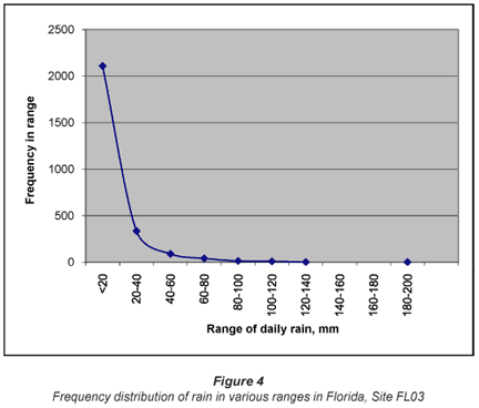
The 2nd data set was collected daily over a period of 30 years between October 1978 and January 2008 at the NADP site FL03 Bradford Forest, (29.9748ºN, -82.1978ºW, and 44 m a.m.s.l.). This was typical of the daily data collected by the NADP (NADP, 2007b). There were 2 597 validated non-zero days of rainfall during this period and 7 393 d of zero recorded rain. The records were essentially continuous except for a gap of 63 d between 17 Jan and 21 March 2006. Two samples were taken every 7 d, one typically from 05:00 to 18:00 and the next from 18:00 to 05:00 the following day. The 2 samples were therefore pooled so that all samples represented a full day, generally from 05:00 to 05:00.
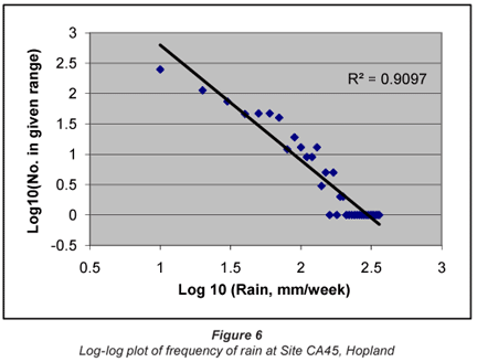
The 3rd data set used to examine rainfall distribution was collected weekly over the period between October 1979 and January 2008 at the NADP site CA45 Hopland (39.0045ºN, -123.086ºW, and 253 m a.m.s.l.). There were 744 validated non-zero records during this period.
The final data set was also collected weekly from December 1981 onwards at the NADP Site CA99 Yosemite, 37.7961ºN, -119.8581ºW and 1 393 m a.m.s.l. There were 681 validated non-zero records during this period.
The distributions of each set of data were determined by sorting into ascending order and straightforward decomposition into classes.
The distribution of rainfall
The instantaneous (5 min) data distribution is shown in Fig. 1. The records for 0.2 to 0.6 mm are omitted as the abscissa scale then becomes so large that the form of the distribution is hidden. Note that the omission is purely for illustrative purposes; the ~6000 records in the 0.2 to 0.6mm range were included in the later analysis. Note also that while points are shown, the numbers on the ordinate are in fact the upper bounds of ranges. So a point shown as 2.0mm rain in 5 min is strictly the range >1.8 <2.0 mm. Again, for clarity, the range is omitted. The same practice is followed in most distributions shown in the rest of this paper.
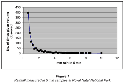
When the data are re-plotted on logarithmic co-ordinates, as shown in Fig. 2, there is a very clear relationship between 5 min rainfall and frequency, as shown in Fig. 2. Figure 2 includes the data which had been omitted for clarity in Fig. 1.

Over nearly 2 orders of magnitude of measured rainfall, and 4 orders of magnitude of frequency, a linear log-log relationship is observed with a regression coefficient of 0.9625, significant at the 0.1% level.
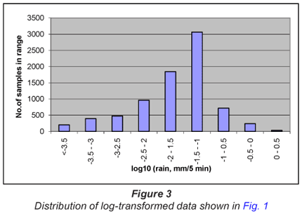
In Fig. 2, the data ranges are selected from the untransformed data. When the data ranges are selected from the log-transformed data, the distribution approximates that of the familiar normal distribution, as illustrated in Fig. 3.
The distribution of the daily rainfall in Florida is shown in Fig. 4. The distribution is clearly not a normal distribution.
However, the frequency of the logarithm of the daily rainfall is again linear with a significant correlation coefficient, as shown in Fig. 5.

The 3rd data set, that from Site CA45, Hopland in California, plotted in a manner similar to that in Fig. 2, also gave a linear log-log relationship between volume and frequency, as shown in Fig. 5. In this case the correlation is poorer than in the case of the 5 min measurements given in Fig. 2, but this may well be caused by the fact that there are far fewer weekly data than there are in the case of the 5 min samples.
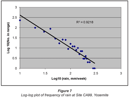
The final data set, that also of weekly rainfall, from Site CA99, Yosemite, showed a very similar distribution, linear in the log domain.
It is therefore clear that rainfall data are, to a close approximation, log-normally distributed, and that any trends should be determined using log-transformed data. It is also apparent that, once transformed, normal statistics may be employed to evaluate any trends and to determine the confidence limits on those trends. The frequency plots also give a reasonable estimate of the probability of very high precipitation events. Figure 2, for instance, shows a real likelihood of 10 mm in 5 min; Fig. 5 shows that over 200 mm/d is likely in Florida; and Figs. 6 and 7 indicate that events of over 400 mm/week are perfectly possible in California.
The estimation of temporal trends
The distribution of daily rainfall records from Florida as a function of time is shown in Fig. 8. Also shown are the trends determined on the entire data set by regression on the untransformed data ('Raw data') and on the log-transformed data ('Linear (Log10)').
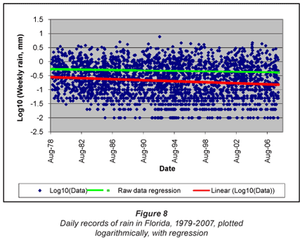
In this one can clearly see a discrete rather than continuous distribution at the lower end (<0.1 mm) of rainfall, which reflects measurement to an accuracy of 0.01 mm. A logarithmic model is therefore by no means perfect, but as we have seen in the previous section, it represents the data to a very good approximation.
There is a definite difference between the regressions in the linear and logarithmic domains. The regression in the linear domain shows a slight downward trend over the period, but it is clearly incorrect to use linear regression on the untransformed data, for the very reasons clearly identified by Sen (1968). In contrast, the regression in the logarithmic domain reveals an obvious trend. The question is what exactly this trend means.
Clearly the noise in the data is such that, at any one point in time, the regression is a very poor estimator of the value at that point in time. But trends are not concerned with values at points in time, but with the change in the mean value over time.
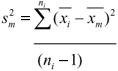
In essence, one is seeking a measure of the change in the sample mean, the variance of which, sm2, will be given by:
If the degrees of freedom, n, are large, then the variance of the sample mean will be far smaller than the variance of the individual sample. Thus the slope of the regression line can indeed estimate how the sample mean changes locally. And it is the slope which gives the desired trend. There is no need to filter the data in any way; no need to be concerned with a poor level of correlation between seasons; and even quite large gaps in the data can be accommodated without seriously affecting the significance of the slope so determined.
There are 2 possible tests for the significance of the regression, namely the F-test and the t-test. Table 1 gives the calculation of F.

The value of F is so high, and the significance so low, that there can be no doubt that the trend in the data is real.
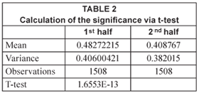
The t-test, comparing the 1st and 2nd halves of the data, gives an even greater significance:
The regression line is of the form:
log10 (rain) = 0.16482-(2.4955x10⁻⁵).D
where:
D is the time in days after 1-01-1900
For the Florida data, the change in rain over the period sampled is given in Table 3.
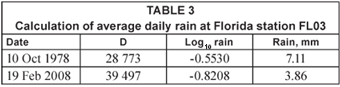
Obviously, there are large errors in these estimates of the average rain, but the trend is obvious – there has been a significant drop at this station. Other stations in Florida have shown an equally significant increase in rainfall.
Several questions may be asked. For instance, is this an artefact of the choice of end dates? The answer is 'no.' It was quite simple to repeat the analysis with subsets of the data, with start dates and end dates at different times of the year. While there is limited seasonality at this station, on average winter tends to be drier than summer, but a significant decreasing trend over the sample period was shown whether the period started in winter and ended in summer, or vice versa. Was there any impact from the missing 3 months? Changing the end date by over 2 years, to October 2005, dropped the value of F to 29.3434, with a slight drop in the significance to 6.66E-08, both of which are negligible considering that about 10% of the data were ignored.
The 3rd set of data was the monthly NADP data from the Californian Site CA45, Hopland. The linear data, smoothed by averaging over 7 successive weeks, are shown in Fig. 9. It is clear that this has a marked seasonality, with winter rainfall sharply higher than that in summer.

Some idea of the difficulty of accounting for seasonal effects may be gained from the fact that the peak rainfall, 39 mm, in February 1994, was close to the minimum, 34 mm, in June 2005. While the peaks look sharp, they occur as early as October and as late as March. It is for these reasons that attempts to correct for seasonality are plagued with difficulties.
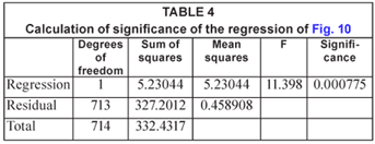
Repeating the exercise with a logarithmic plot of the data for Hopland gives the picture shown in Fig. 10, with a very clear trend of increasing rainfall.

The F-test of this data shows that this trend is highly significant, as illustrated in Table 4. The level of significance is somewhat lower than in the case of the daily data because the sample size is so much smaller.
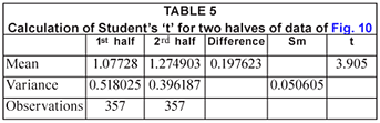
The average rainfall increased from about 10.8 to 21.4 mm/week over the sample period, although again it must be noted that there are large statistical errors on both these estimates. However, the increase was again statistically significant in terms of the t-test as shown in Table 5 – a value of 't'>3.9 is significant at the 99.95% level.
The final set of data, from Site CA99 Yosemite, is shown in a logarithmic plot in Fig. 11. In this case it seems doubtful whether a trend exists – there may be a slight increase in rainfall over the period, but the slope of the regression line is not nearly as marked as in earlier cases.
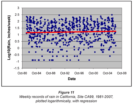
An F-test of the data confirms the visual impression, that there is no significant trend over the period, as shown in Table 6.
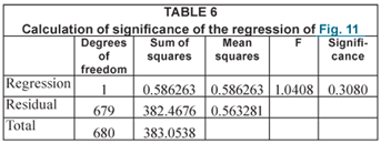
The significance indicates that there is >30% chance that any trend shown arises from random effects. In this case, however, the t-test estimates that the trend is significant at the 98% level. This would seem, on the available evidence, to be a case of a false positive.
Discussion
A number of attempts to employ published methods to determine trends in rainfall data failed. It was noted, however, that no one appeared to have examined the underlying distribution of the data, but had set about the analysis as if the distribution were of no moment.
When a number of data sets were examined, a clear logarithmic signal appeared. The sort of log-log relationship shown in Fig. 2 has re-appeared in a number of guises. This would appear important from the point of view of flood prediction – given such a linear relationship, the likely upper limits on the rate of precipitation emerge directly. Of course, it is difficult to imagine widespread use of recording gauges such as that employed to generate the data from which Fig. 2 was derived, but all the data show a similar pattern.
This underlying logarithmic relationship carries through to the frequency distributions such as illustrated in Fig. 6. What these imply is that one cannot employ normal statistics to evaluate trends in rainfall – arithmetic means have no useful purpose when assessing distributions such as those in Fig. 3. The arithmetic mean cannot tell what the most likely condition will be, nor what the likelihood of an extreme event may be. One is forced to use a distribution such as the logarithmic, in which there is a closer relationship between the most likely (modal) and average event, and where the standard deviation gives a reasonable idea of the magnitude of the extreme event.
This, of course, calls into question the usual method of reporting the quantity of precipitation as an arithmetic average. On statistical grounds, use of a geometric average is much to be preferred, as the arithmetic average of log-normally distributed data is biased high. To do so would mean discarding several centuries of data, so that such a step is probably impractical. It does, however, merit serious consideration, as a high bias can lead to planning errors and the under-provision of water supplies.
Repeated testing on a wider range of data than it has been possible to consider here has shown the utility of this approach. It appears robust – when an F-test of the log-transformed data indicates a trend, other measures will usually confirm it, whereas those other measures may either miss a trend or indicate one that is not in fact present, as in the example given here for the data of Site CA99. It also appears reasonably sensitive. The method was applied to data from 154 stations, and gave significant (>90%) increases in rainfall at 28 stations, significant decreases at 55, and no significant change at 71, over the period January 1984 to December 2006. If the estimated change in the log-mean rainfall was ~10%, in 70% of the cases the change was significant. If the estimated change was ~20% or greater, in every case it was highly (>99%) significant.
These findings largely follow on from those of Hess et al. (2001), except that work focused on the application of linear regression to the linear domain. One of the difficulties of such an approach is that any attempt to extrapolate a falling trend must ultimately lead to negative values, something which is impossible in the logarithmic domain.
The methodology has the additional benefit of not requiring corrections for seasonality. As long as the data are reasonably continuous, changes with season are merely another source of noise.
Importantly, simplicity has great charm. The experience gained with attempts to determine trends using both parametric and non-parametric methods, or of employing filters, was salutary indeed. Dealing directly with cold, hard, raw data became a pleasurable experience after hacking through those woods.
Conclusions
The log-transformation of rainfall data gives rise to a distribution that is reasonably close to normal, so that normal statistics can be applied reliably to the transformed data. In contrast, the very skew nature of the untransformed data makes normal statistics inapplicable. This has given rise to a range of methods which this study found to be of doubtful utility, confirming the earlier findings of Hess et al. (2001). Both the F-test and t-test to determine the significance of the trend gave good measures of the significance of the trends observed. It must be stressed that it is the trend which is robust, effectively the slope of the line of the regression, and not the value of the variable at any point along the trend, which, because of the noisy signal, has a high variance associated with it. The frequency distributions also are linear, which suggests a method for estimating the maximum rate of precipitation, although this has not been widely tested in this work.
Acknowledgements
I must thank Dr W Nel, of the University of Fort Hare, for making available to me the continuous sample data set from Royal Natal National Park and similar sets not quoted here. Various members of the NADP team, including VC Bowersox and SM Larsen, have offered valuable advice and answered many questions. Stephen Davis, of the Energy Research Centre, made some useful comments on the statistical aspects. Three referees who made most constructive comments on the original draft are to be thanked for their diligence.
References
BRILLINGER D (1989) Consistent detection of a monotonic trend superposed on a stationary time series. Biometrika 76 23-30. [ Links ]
CHENG K-S, HSU H-W, TSAI M-H, CHANG K-C and LEE R-H (2004) Test and analysis of trend existence in rainfall. Proc. Asia Pacific Assoc. Hydrology and Water Resources. 5-8 July 2004, Singapore. Paper No.56. http://www.wrrc.dpri.kyoto-u.ac.jp/~aphw/APHW2004/proceedings/OHS/56-OHS-A527%20(PDF%20only)/56-OHS-A527.pdf (Accessed August 2008). [ Links ]
CIVEROLO K and RAO ST (2001) Space-time analysis of precipitation-weighted sulphate concentrations over the eastern US. Atmos. Environ. 35 5657-5661. [ Links ]
GILBERT RO (1987) Statistical Methods in Environmental Pollution Monitoring. Van Nostrand Reinhold, New York, USA. [ Links ]
HELSEL DR and HIRSCH RM (1992) Statistical Methods in Water Resources. US Geological Survey, Reston, VA. [ Links ]
HESS A, IYER H and MALM W (2001) Linear trend analysis; a comparison of methods. Atmos. Environ. 35 5211-5222. [ Links ]
HIRSCH RM, SLACK JR and SMITH RA (1982) Techniques of trend analysis for monthly water quality data. Water Resour. Res. 18 107-121. [ Links ]
LEHMANN CMB, BOWERSOX VC and LARSON SM (2005) Spatial and temporal trends of precipitation chemistry in the United States, 1985-2002. Environ. Pollut. 135 347-356. [ Links ]
LEHMANN CMB, BOWERSOX VC, LARSON RS and LARSON SM (2007) Monitoring long-term trends in sulfate and ammonium in US precipitation: Results from the National Atmospheric Deposition Program/National Trends Network. Water Air Soil Pollut. Focus 7 (1) 59-66. [ Links ]
McLEOD AI, HIPEL KW and BODO BA (1991) Trend analysis methodology for water quality time series. Environmetrics 2 169-200. [ Links ]
MILLARD S P and NEERCHAL N K (2000) Environmental Statistics with S-Plus. CRC, Boca Raton, USA. 680-685. [ Links ]
NADP 2007a (NRSP-3) NADP Program Office, Illinois State Water Survey, 2204 Griffith Dr., Champaign, IL 61820. [ Links ]
NADP (2007b) http://nadp.sws.uiuc.edu/ (Accessed Jan-July 2008). [ Links ]
NEL W (2008) Personal Communication, May 2008. University of Fort Hare, Eastern Cape, South Africa. [ Links ]
NEL W and SUMNER PD (2008) Rainfall and temperature attributes on the Lesotho-Drakensberg escarpment edge, southern Africa. Geogr. Ann. 90 A (1) 97-108. [ Links ]
PARK J-S, JUNG H-S and CHO S (2000) The instrumental precipitation records during the last 220 years in Seoul, Korea. http://isi.cbs.nl/iamamember/CD2/pdf/722.PDF (Accessed August 2008). [ Links ]
PETTITT AN (1979) A non-parametric approach to the change-point problem. Appl. Stat. 28 (2) 126-135. [ Links ]
RAO ST and ZURBENKO IG (1994) Detecting and tracking changes in ozone air quality. J. Air and Waste Manage. Assoc. 44 1089-1092. [ Links ]
REINSEL GC (1989) Trend analysis of aerosol-corrected Umkehr ozone profile data through 1987. J. Geophys. Res. 94 16373-16386. [ Links ]
REINSEL GC and TIAO GC (1987) Impact of chlorofluoromethanes on stratospheric ozone. J. Am. Stat. Assoc. 82 20-30. [ Links ]
REINSEL GC, TIAO GC, WANG MN, LEWISR and NYCHKA D (1981) Statistical analysis of stratospheric ozone data for trend detection. Environmetrics 81 Selected Papers, 215-235. [ Links ]
SEN PK (1968) Estimates of the regression coefficient based on Kendall's tau. J. Am. Stat. Assoc. 63 1379-1389. [ Links ]
TIAO GC (1983) Use of statistical methods in the analysis of environmental data. Am. Stat. 37 459-470. [ Links ]
WIDMANN M and SCHAR C (1997) A principal component and long-term trend analysis of daily precipitation in Switzerland. Int. J. Clim. 17 (12) 1333-1356. [ Links ]
Received 1 August 2008; accepted in revised form 19 March 2009.
* To whom all correspondence should be addressed.
+2721 650 3896; fax: +2721 650 2830;
e-mail: Philip.Lloyd@uct.ac.za

