First steps in the development of a water temperature model framework for refining the ecological Reserve in South African rivers

 

 

NA Rivers-Moore^{I, *}; DA Hughes^I; S Mantel^I; TR Hill^II

^IInstitute for Water Research, Rhodes University, PO Box 94, Grahamstown 6140, South Africa
^IIDiscipline of Geography, School of Environmental Sciences, University of KwaZulu-Natal (Pietermaritzburg), Scottsville 3209, South Africa

 

 

---

ABSTRACT

Ecological Reserve determination for rivers in South Africa presently does not include a water temperature component, in spite of its importance in determining species distribution patterns. To achieve this requires an understanding of how lotic thermographs from South African rivers differ from northern hemisphere rivers, to avoid mismanaging rivers based on incorrect regional assumptions. Hourly water temperatures from 20 sites in four river systems, representing a range of latitudes, altitudes and stream orders, were assessed using a range of metrics. These data were analysed using principal component analyses and multiple linear regressions to understand what variables a water temperature model for use in ecoregions within South Africa should include. While temperature data are generally lacking in low- and higher-order South African rivers, data suggest that South African rivers are warmer than northern hemisphere rivers. Water temperatures could be grouped into cool, warm and intermediate types. Based on temperature time series analyses, this paper argues that a suitable water-temperature model for use in ecological Reserve determinations should be dynamic, include flow and air temperature variables, and be adaptive through a heat exchange coefficient term. The inclusion of water temperature in the determination and management of river ecological Reserves would allow for more holistic application of the National Water Act's ecological management provisions. Water temperature guidelines added to the ecological Reserve could be integrated into heuristic aquatic monitoring programmes within priority areas identified in regional conservation plans.

Keywords: water temperatures, conservation planning, water temperature modelling, management

---

 

 

Introduction

Global ecosystems face unprecedented crises in habitat fragmentation, destruction and ultimately extinction, and of all the varying ecological systems rivers are the most neglected and endangered (Groves, 2003; Driver et al. 2005; Roux et al., 2005.). The greatest threat to these systems is the loss or degradation of natural habitat and processes, and water temperatures, after flow volumes, are a primary abiotic driver of species patterns within river systems (Driver et al., 2005). Stuckenberg (1969) highlighted the links between temperature, topography and faunal assemblages, while Rivers-Moore et al. (2004) highlights the major impacts of water temperatures on organisms and illustrate how water temperatures are one of the primary environmental drivers structuring fish communities in the Sabie River, arguably the most ichthyologically species-rich river in South Africa.

Taking cognisance of the crisis faced in managing lotic resources, current conservation planning aims to maintain not only biological diversity, but also the ecological and evolutionary processes which ensure the continued positive functioning of such systems (Groves, 2003). This can only be achieved through a thorough understanding of these processes, and in defining conservation goals and objectives. However, Tear et al. (2005) point out that it remains difficult to set quantitative targets. Without targets, the objectives of systematic conservation planning, representation, redundancy, and resilience of ecosystems (Margules and Pressey, 2000), with an inherent recognition of the need to preserve processes and system variability are unattainable. In conservation planning, the 'range of variability' or 'natural range of variation' approach has been advocated as a useful tool in adaptive management for setting flow targets (Richter et al., 1997; Groves, 2003), and the role of disturbance and variability is recognised in maintaining diversity (Richter et al., 1997). To attempt such an approach both temporal and spatial dimensions need to be specified to take into account nested geographical and seasonal variation. To apply this requires that the time scale and geographical area are first specified (Groves, 2003), while analyses are typically based upon frequency distributions of physical and biological conditions. Temperature is a continuous climatological variable, which is both temporally and spatially conservative, such that record lengths do not need to be as long as for other variables (such as precipitation) to evaluate time series with confidence (Schulze and Maharaj, 2004).

The National Water Act (Republic of South Africa 1998) provides legal status to the quantity and quality of water required to maintaining the ecological functioning of river systems, through the declaration of the 'ecological Reserve' (see Chapter 3, Part 3 of the National Water Act of 1998). To date, no methods have been developed for the water temperature component of the Reserve, although the importance of water temperatures in maintaining river systems is fully recognised (Poole and Berman, 2001; Johnson, 2003). Understanding temporal variability of temperature time series, regional variation, and how aquatic macroinvertebrates respond to thermal regimes both spatially and temporally, is central to determining ecological Reserves, and in defining policies to manage river systems.

The extent to which South Africa's rivers have their own distinct thermal characteristics is largely unknown. Ward (1985) concluded that what makes southern hemisphere rivers distinct from northern hemisphere rivers is 'a matter of degree rather than of kind', i.e. South African rivers may have parallels in the northern hemisphere, but a greater proportion of these will be more variable than in the northern hemisphere. Chiew et al. (1995) have demonstrated that southern African rivers, like Australian rivers, have extreme flow regimes, displaying twice the world average of flow variability. This variability is reflected in their thermal and hydrological regimes, and Basson et al. (1994) recognised that such system variability between months in southern hemisphere regions presented management and simulation challenges not present in northern hemisphere regions. A concern is that we are presently utilising northern hemisphere research findings (for example Eaton and Scheller, 1996; Essig, 1998; Poole and Berman, 2001), which purport the ecological importance of water temperature, as the basis for detecting system change in South Africa's rivers.

To apply a similar approach within the South African aquatic management community would require time series data to a higher degree of confidence which is often not locally available due to a paucity of data. Primary constraints are the lack of long time series and insufficient temperature monitoring points. In the absence of time series, scenario analyses assume greater importance, and this requires sound predictive models. Models, such as the expert system for assessing the conservation status of rivers developed by O'Keeffe et al. (1987), are powerful tools in evaluating rivers at a landscape scale under varying environmental scenarios. From these foundations, it has been recognised that a higher level of resolution and the importance of simulating specific environmental variables (temperature) is required as a subsequent progression from such earlier systems as the adaptive management approach has developed. Consequently, the need exists for water temperature models as necessary management tools in simulating water temperatures, particularly in cases where observed data are scarce, where surrogate driver data are available, and in situations where decision-makers are concerned with environmental scenario analyses (Rivers-Moore and Lorentz, 2004). As a consequence of the general dearth of water temperature data, simulation modelling of water temperatures, with associated scenario analyses, is the most suitable approach to incorporating water temperatures into ecological Reserve determination studies. The utility value of this approach increases when this is related to spatial elements, such as the South African ecoregion approach (Kleynhans et al., 2005), where the landscape is classified into units of similar abiotic components which act as biotic surrogates.

The aim of this paper is to characterise water temperature time series in selected South African rivers, compare these with northern hemisphere rivers and provide a conceptual water temperature modelling approach for South African Rivers, which would feed into the ecological Reserve process.

 

Methods

Quantifying temperature trends in South African rivers

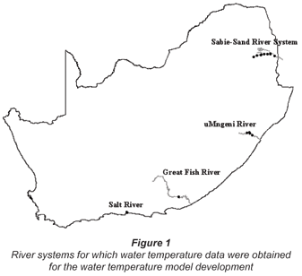
Temperature time series from 20 sites in four sampled river systems (Table 1 and Fig. 1) were analysed to provide preliminary insights into thermal signatures in selected South African river systems. Water temperature sites covered a range of stream orders and river latitudes and altitudes. The geographical location of data sites is illustrated in Fig. 1. Hourly water temperatures for the Salt River (Western Cape) represent an unregulated river system with a unique aquatic invertebrate fauna (De Moor, 2006). Thirty-two months of hourly water temperature time series for the Sabie-Sand River system, an unregulated highly variable system, were available from Rivers-Moore et al. (2004), while one year of hourly water temperatures were recorded from a single site on the Great Fish River, a regulated river system (Rivers-Moore et al., 2007). Finally, 6 months of hourly water temperatures for 4 sites on the uMngeni River, a regulated river, were obtained from Dickens et al. (2007).

 

 

 

 

Daily temperature statistics (mean, maximum) were calculated from the hourly water temperature time series. To help develop an understanding as to how water temperatures in South African rivers may differ from water temperatures in northern hemisphere rivers, maximum daily range and cumulative degree days per month as agglomerative/descriptive metrics were used, and related to stream order, after Vannote and Sweeney (1980). Stream orders were assigned according to Strahler's (1964) stream ordering system (Chow et al., 1988). This provided a broad basis, supported by selected literature on water temperatures from northern hemisphere river systems (North American rivers – see Vannote and Sweeney, 1980), with which to compare southern hemisphere water temperatures.

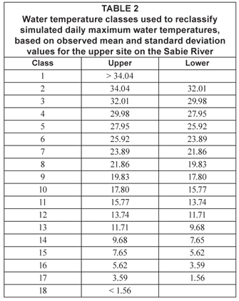
Predictability of water temperatures in relation to stream order were calculated using Colwell's (1974) predictability indices. Daily average water temperatures were reclassified into water temperature classes (Table 2), based on n successive standard deviations on either side of the mean for observed water temperatures in the upper Sabie catchment. This site was chosen since it exhibited the least variability of the nine sites surveyed in the Sabie River system. Colwell's (1974) indices of predictability (p), constancy (c) and contingency (m) values were calculated for each site, based on the contingency tables.

 

 

The percent contribution made to predictability either by constancy or contingency was calculated by dividing the predictability value by either index. A fundamental requirement of any data for use in Colwell's (1974) indices, particularly involving phenomena with fixed lower bounds, is that the standard deviation and mean are uncorrelated (Colwell, 1974). For example, with data that have a fixed lower bound (0), such as hydrological data, there is often a high correlation between mean and standard deviation. While in practice water temperatures do not generally have a fixed lower bound, these data were tested for correlations between annual mean and standard deviation, since a high correlation between the mean and standard deviation necessitates a log transformation.

Assessment of model variables

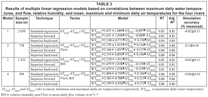
Multiple linear regression modelling was undertaken to determine which driver variables contributed most to water temperature signatures. Four suites of models to predict maximum daily water temperatures, based on combinations of variables (daily air temperature metrics – °C; mean daily flow – m³·s^-1; relative humidity – % – see Table 3) were developed using standard, stepwise forward and stepwise backward techniques (StatSoft 2003). As the dataset from the Sabie River was the largest, half of these data (February 2001-September 2002) were used for developing the model (in addition to all data from the Great Fish, Salt and uMngeni Rivers). The latter half of the Sabie River data (October 2002 and October 2003) was used for assessment of the four models, with model accuracy calculated as the mean (± standard deviation) percentage difference between observed and simulated maximum daily water temperature. In these models, the assumption was made that the use of broad datasets from a range of location would make a more robust model for South Africa, in spite of geographical differences, which were assumed to be secondary to model robustness.

In addition, the 20 sites in the four river systems (11 470 water temperature records) were characterised by the 16 variables listed below:

• Annual mean temperature

• Annual standard deviation

• Annual coefficient of variability

• Predictability (Colwell, 1974)

• Absolute minimum

• Absolute maximum

• Mean daily minimum

• Mean daily maximum

• Average diel range

• Maximum diel range

• Mean spring temperature

• Mean summer temperature

• Mean autumn temperature

• Mean winter temperature

• Julian date of annual minimum

• Julian date of annual maximum.

Prior to undertaking a principal components analysis (PCA), correlations between variables were tested to eliminate redundant variables (StatSoft 2003). A PCA was performed using PC-ORD (McCune and Mefford, 1999) to determine which variables had the greatest influence on structuring site clusters. In this analysis, a correlation matrix was used, since there was little 'a priori basis for deciding if one variable is more ecologically important than the other'(McGarigal et al., 2000). Site groupings were also examined using cluster analysis techniques to assist in the interpretation of PCA scatter plots (Euclidean distance measure; un-weighted pair-group averages) (McCune and Mefford, 1999).

 

Results

Southern vs. northern hemisphere trends

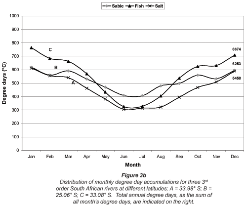
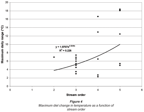
Total annual degree days in the four river systems ranged from 5200 to 8700°C, with a difference of 3500°C (Fig. 2). In the 2^nd to 5^th stream orders, the winter months exhibited the lowest monthly degree day accumulations, with monthly accumulations ranging between 300 and 900°C. In general, monthly degree day accumulations increased with stream order and showed an inverse relationship with altitude (Fig. 3a), while the relationship was not as marked for latitudinal gradients (Fig. 3b). Maximum diel change increased exponentially with stream order (Fig. 4), but this relationship was weak (R² = 0.23), with few data points for low order streams. It appears that maximum diel range increased in variability with stream order.

 

 

 

 

 

 

 

 

The correlation between the mean and standard deviation for the calculated water temperatures was non-significant (p < 0.01), and untransformed temperature data were consequently suitable for subsequent classification using Colwell's indices. Predictability decreased with stream order (Fig. 5), inferring that upper catchment rivers and tributaries had more predictable water temperature regimes than higher order rivers. However, these data showed greater variability in the mid-order streams than in the higher and lower order streams.

 

 

Model variables

All four multiple linear regression model sets assessed, based on standard, stepwise forward and stepwise backward methods, provide similar results. The air temperature parameters (mean and minimum daily air temperatures) were significant, while the flow and relative humidity terms were not significant and were therefore excluded from the models (Table 3). Model verification showed that predictions of maximum daily water temperature improved with increase in sample size.

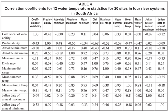
Correlation analyses showed that mean minimum and mean maximum daily water temperatures were highly correlated with annual mean water temperatures (R² = 0.98). Mean maximum water temperature was highly correlated with mean summer and mean autumn water temperatures (R² > 0.96). For pragmatic reasons, mean maximum and annual mean water temperatures were therefore excluded from the principal components analyses. As standard deviation of annual water temperature was used to derive the coefficient of variability; this variable was excluded from further analyses. Mean spring water temperatures were also excluded from the analyses, since values could not be calculated for all sites. The correlation matrix of the remaining 12 variables is provided in Table 4.

 

 

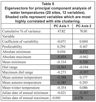
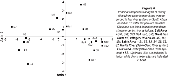
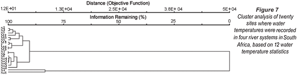
The first two principal component axes accounted for almost 71% of the variability between sites. Eigenvectors are presented in Table 5. From these analyses, the variables absolute maximum, diel range, mean summer temperature and mean autumn temperature contributed most to the site weightings in Axis 1, and exhibited a negative gradient with site groups. For Axis 2, absolute and mean minimum water temperatures were highly positively correlated with site groupings, while maximum temperature range and Julian date of annual maximum and minimum were highly negatively correlated with site groupings. A scatter plot of the principal components analysis is shown in Fig. 6, which showed three clear site groupings. Used in conjunction with the cluster analysis (Fig. 7), sites could generally be grouped into a warmer, downstream (lowveld) assemblage (S7, S6, S5, SS), a cooler upstream group (S1 and Salt River (Sa) sites), and an 'intermediate' middle reach grouping. Sites were also characterised by their level of predictability, even though this variable contributed less (0.294) to the weightings in Axis 1 than those weightings already mentioned, because of the importance of predictability to biological patterns (Colwell, 1974; Vannote and Sweeney, 1980). The warmer assemblage exhibited high summer and autumn water temperatures, high temperature extremes (high absolute maximum and diel range) and lower predictability. Conversely, the cooler upstream group was characterised by more predictable, cooler and less extreme water temperatures. The intermediate group showed higher absolute and mean minima, and an associated lower maximum range. This was also manifested in earlier onset of cool winter minima (Lower Julian annual minimum), which was approximately in June for the uMngeni and Fish River sites, in August for the Salt River Sites, and July/August for the Sabie River sites. The cluster analysis showed the sites Sa1 (Salt River upstream site) and S4 (Sabie River) to be distinct from the remaining sites at the first level of separation (Fig. 7). The larger group could be divided further into generally downstream (warmer) vs. upstream (cooler) sites at a second level of separation. The warmer group could be further split based on lower vs. lower reach sites, while the cooler group split into a pool site vs. the remaining non-pool sites.

 

 

 

 

 

 

Discussion

Southern vs. northern hemisphere differences

Compared to the figures of Vannote and Sweeney (1980) (Table 6), there are indications of variation between northern and southern hemisphere river water temperatures. All rivers in this study were warmer than those by Vannote and Sweeney (1980), even though the rivers considered in both studies were at comparable latitudes. However, while the lower order streams in this study had lower temperature amplitudes than the higher order streams, as found by Vannote and Sweeney (1980), they were generally cooler than the higher order streams, while in the study by Vannote and Sweeney (1980), the lower order streams generally remained warmer in winter due to groundwater inputs. One generalisation is that amplitude in degree days increases with stream order, as does maximum range in diel temperatures. A data gap in South African water temperatures is that little is known about groundwater impacts on water temperatures; Vannote and Sweeney (1980) reported that streams with high groundwater inputs are less variable than streams dominated by surface runoff, and that groundwater-fed streams have more stable temperatures throughout the year, i.e. cooler in summer and warmer in winter. While the South African data differ annually by over 3 000 degree days, with low order streams having much lower annual degree days than higher order streams, the figures of Vannote and Sweeney (1980) showed a difference of only 62 degree days between first and third order streams, with all values being similar (4 222 to 4 284). However, like Vannote and Sweeney's (1980) findings, diel variation increases with stream order.

 

 

In this study, no data were obtained to test whether this variation again decreases after 5^th order streams, as was reported by Vannote and Sweeney (1980). South Africa has relatively few 'large', higher order rivers, with the Orange River being one notable exception. There are particular gaps in data for first-order streams, as well as in higher-order streams (5^th order and above). Additional data from targeted river systems, both regulated and unregulated (as far as possible) are required, and preferably for at least one full year, before further general patterns can be highlighted. From these data there are indications that water temperatures in regulated rivers are more predictable than in unregulated rivers, although these estimates are not based on a full annual temperature cycle.

All rivers in South Africa would be classified as temperate (23.5 to 66° latitude) (according to Ward, 1985). One important difference between southern and northern hemisphere rivers is that most temperate northern hemisphere rivers drop to 0°C during winter unless they are groundwater-fed. This difference is largely due to the latitudinal differences in the distribution of land masses, with northern hemisphere rivers also flowing through much higher latitudes than South African rivers. Despite its importance in northern hemisphere rivers, surface and subsurface ice is of very little importance in the ecology of southern hemisphere rivers (Ward, 1985). South Africa's highly variable rivers, with associated extreme flow fluctuations, typically have extreme temperature fluctuations, with marked year-to-year differences in thermal regimes (Ward, 1985). These data support this contention, with maximum diel range increasing, and predictability decreasing, with stream order. Lake (1982), in describing highly variable Australian river systems, hypothesised that unpredictable thermal regimes would have insects with flexible life histories, and flexible communities lacking highly synchronised species complexes. This decreasing predictability of water temperatures has important consequences for biota and their associated life histories (De Moor, 2006).

Model variable assessment – towards a conceptual model

Confirming the findings of this study, air temperature has been shown to be the most sensitive driver variable for water temperatures (Bartholow, 1989). However, the effects of air temperatures on water temperatures are buffered by a combination of flow and residency times (width: depth ratios) (Bartholow, 1989).

The results demonstrate that distinct thermal differences existed between upper and lower reaches, which was borne out by the principal component analysis (PCA). Notably, cumulative monthly water temperatures in the upper reaches of the rivers considered (Salt River, upper Sabie River) showed less seasonality (flatter curves) than in the lower river reaches (Fish River, lower Sabie River) (Fig. 2). It was assumed that greater groundwater inputs in the upper reaches resulted in more stable thermal regimes with less seasonal effects. Conversely, water temperatures in the lower reaches are more influenced by thermal radiation, and show more marked seasonality than water temperatures in upper river reaches. An additional compounding factor could be the change in cross-sectional profiles down the longitudinal axis of a river, where wider, shallower rivers in lower reaches are exposed to greater amounts of solar radiation than shaded, incised rivers in upper reaches.

Site groupings in the PCA suggest that an ecoregion approach to predicting water temperatures would be appropriate. Data also suggest that temperature extremes (mean and absolute maxima and minima; daily range) are important in site-specific water temperature signatures, and that any water temperature model would need to take cognisance of this. Finally, the date of winter minima is more variable (June to August) than the onset of summer maxima (February), suggesting that winter temperatures are important in determining local site characteristics, and determining species community patterns and turnover in time and space (Vannote and Sweeney, 1980). Thus, an ecologically suitable water temperature model should focus not only on daily maximum water temperatures, but also daily minimum water temperatures, which could provide insights into understanding the magnitude and direction of energy fluxes influencing water temperatures (Johnson, 2003).

Correlations between air temperatures and water temperatures were shown to be the most significant predictor of water temperatures (Steffan and Preud'homme, 1993). Multiple regression models suggest that the effects of relative humidity, rainfall and flow are small compared to air temperatures (current analyses, but see also Webb and Nobilis, 1997; Rivers-Moore et al., 2005). It would appear that no single generic statistical model is possible, since relationships typically vary between catchments (Webb and Nobilis, 1997; Rivers-Moore et al., 2004). Such a complex relationship was also demonstrated for the Sabie River (Rivers-Moore et al., 2004; Rivers-Moore et al., 2005), where each of 9 sites' water temperatures could best be simulated by a unique multiple regression model, and that site-specific simulation accuracy was reduced when a single generic model was applied.

This study demonstrated that each river site tends to be unique, such that were a statistical modelling approach adopted, a unique model would need to be developed per site, which is logistically not feasible. The highest correlations were achieved using multiple linear regression models which did not incorporate a flow-dependent term. However, the incorporation of a flow term, while reducing model accuracy, greatly enhances the utility value of such a model (Rivers-Moore et al., 2005), because of the increased model utility to aquatic ecologists and engineers in predicting the consequences of different flow modification scenarios on water temperatures. The results of this study showed, in addition to the overriding influence of air temperatures as a surrogate for solar radiation, that model accuracy increased with increasing sample size. Ongoing development of a water temperature model should thus proceed in conjunction with ongoing collection of sub-daily water temperature data, and associated data on water temperature buffers, including, inter alia, turbidity and cross-sectional profiles.

The results suggest that the following components are important to the development of a water temperature model:

• Solar radiation (air temperatures as surrogate) will be a major driver

• The model should be spatially dynamic and flexible enough to incorporate upstream-downstream effects (see Rivers-Moore and Lorentz, 2004)

• Evaluation of temperature signals needs to be attached to different flow components, i.e. disaggregation of (monthly) flows into groundwater vs. instream (surface and interflow) flows.

The 'ideal' water temperature model should consider the following:

• Use data which are readily and widely available (air temperatures)

• Integrate with other models, and use outputs from these

• Be useful in scenario analyses

• The model time step should be suitable for ecological Reserve application and general ecological use; a daily time-step model would be the most useful for these purposes

• Build on existing research on water temperature models in South Africa

• Generic, i.e. be applicable at a range of spatial scales and applicable throughout South Africa

• Simple, with as few terms as possible

• Dynamic, i.e. allow for simulating change in water temperature with change in downstream distance.

A suitable water temperature model should be flexible enough to incorporate the relative buffering effects of different components of a hydrograph (groundwater and surface water) on water temperatures. Outputs from a suitable model, such as the Pitman Model, which generates three flow parameters (groundwater, surface water and interflow) based on rainfall inputs and evaporation (Hughes, 2004), would provide input data into a water temperature model. A generalised water temperature model should be of the form of Eq. (1), in which flow-weighted heat gains and losses are modified through an exponential modifier term, similar to that used by Walters et al. (2000). One possible approach to simulating the extent of departure from equilibrium temperature is to use (multiple) linear regression models which apply to different ecoregions to estimate regional departures from equilibrium temperatures. These could then be applied to the proposed dynamic water temperature model and applied spatially.

where:

δT° is a change in water temperature with change in downstream distance (δx) is a function of air temperature (AT)

flow1, flow2 and flow3 respectively are groundwater, surface water and interflow components of a hydrograph

c is a heat exchange coefficient dependent on ecoregion geomorphology – for example, the pool/riffle ratio (profile classification) and width: depth ratio, which is in turn modified by flow volume (Q), turbidity (Tb) and riparian shading (Sd)

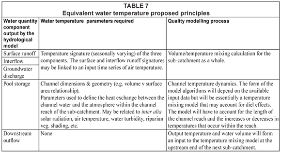
A suitable water temperature model should thus cater for in-stream, in-reach water temperature simulations, driven by air temperatures, and buffered by the effects of turbidity, riparian shading, residency time, and hydraulics. Each of these time series will be used as inputs to simulate downstream water temperatures (i.e. between reach water temperature simulations). Preliminary analyses in this paper suggest the importance of both daily minima and maxima in determining site-specific water temperature signatures, so that an ecologically useful water temperature model should be able to simulate daily mean, minimum and maximum water temperatures. The basic principles of the water temperature model are presented in Table 7.

 

 

Ecological Reserve

In measuring water temperatures, a tradeoff exists between gathering high spatial resolution and high temporal resolution data, and requires developing complementary sampling approaches. In this preliminary analysis, high temporal resolution has been attained for a relatively short time period, while spatial resolution is low. It is possible to record spatially continuous temperature data (for example using forward-looking infrared videography) (Torgersen et al., 2001), and complemented with continuous monitoring using data loggers (Torgerson, 2002, cited in Fausch et al., 2002).

Three steps in the process of 'measuring' river health are to establish baseline conditions, measure departure from the baseline, and implement management action through recognising when thresholds have been exceeded (Ladson et al., 2006). Within this hierarchy, the definition of baseline conditions is critical, since there are a wide range of these depending on the starting point – historical (pre-human; pre-Colonial), least disturbed, best attainable – which all reflect differing degrees of biological integrity (Stoddard et al., 2006). Metrics using aquatic macroinvertebrates can be useful in determining these levels. However, it is becoming increasingly clear in the literature that the way such data are collected and used determines the value of any stream measurements. Specifically, there is criticism of the 'representative reach' approach, which is based on a subjectively chosen stretch of river and does not allow for the estimation of means and standard deviations, nor confidence limits (Ladson et al., 2006; Smith et al., 2005). Alternatively, there is support for randomly selected sites, with the number of sites increasing depending on which measure of river health is required (Ladson et al., 2006), and the development of techniques to assign confidence thresholds to these metrics (Smith et al., 2005). However, random sampling may not be appropriate when particular ecological problems require answers. These emerging approaches and the associated mixed debate are encouraging given that there is an established recognition of the importance of variability within river systems, as well as the need to establish 'natural' ranges of variability. Given that South African river systems have been shown to be highly variable and statistically to be described by extremes, these emerging approaches are particularly pertinent to any use of water temperatures in ecological Reserve determinations.

An initial step in determining the temperature component of the Reserve would be to develop suitable indices for characterising time series of temperatures. Notably, frequency, duration and timing of thermal periods need to be related to different biota, and related to life histories of different species. Indices of predictability, with careful definitions of classes, need to be applied to life history patterns and stability of community structures. This would at least set initial recommended thresholds of variability and seasonality. A critical step is defining these by geographical region. Additionally, the ecological Reserve should also consider the importance of temperature extremes, notably daily maximum water temperatures, as well as their temporal predictability. Given the relationship between water temperature and flow volumes, the ecological Reserve should consider the particular relationship between, and significance of, extreme low flows and water temperature, and flow/temperature-biotic response stressor relationships. This may assist in prioritising future areas of research.

An additional factor useful to the ecological Reserve and water temperatures is the spatial representation of vulnerability to thermal alteration, particularly under anticipated scenarios of global climate change, and/or effects of inter-basin transfer schemes. The approach of Richter et al. (1997), which attempts to describe flow series based on their 'natural' range of variability, is a useful one, particularly when applied spatially (Richter et al., 1998). It is critical that aquatic management aims to preserve as much system variability as possible to protect freshwater biodiversity, with river systems classified regionally based on the key attributes and ranges of variability of component time series (Arthington et al., 2006).

South Africa is a conservation planning 'hotspot' (Knight et al., 2006). Conservation plans should provide a 'scientifically sound, and therefore defensible, basis for land-use decision making' (Knight et al., 2006 p. 5). Setting conservation goals becomes necessary to achieve representation and persistence. To this end, relevant spatially explicit data at the appropriate scales are necessary to identify regions of importance. According to Knight et al. (2006), 'the lack of spatially explicit data on environmental processes is a …hindrance' (p. 6). Spatial layers showing transformation and predicted future pressures are relatively expensive (Knight et al., 2006). However, under conditions of anticipated climate change, this becomes necessary.

Conservation of diversity is often leveraged using targets – % area required to conserve x% of species, based on species-area curves. An equivalent approach in river systems is to use species-discharge curves as a conservation planning tool (Xenopoulos and Lodge, 2006). Flow rates are reduced by water abstractions, as well as anticipated climate change, which in turn will impact on water temperatures. Species-discharge model's predictive power will be increased by the inclusion of other factors in addition to discharge, including water temperatures. A suitable abiotic-biotic predictive framework which links biotic response to changes in flow volumes and water temperature provides the predictive power required by natural resource managers to link species loss (or failure to meet biodiversity conservation targets) to quantifiable flow volumes and water temperature regimes. As an illustrative example, reduced flows lead to increased water temperatures, and increased eutrophication, which in turn facilitates establishment of parasites and fosters infections (Steedman, 1991). Thus, determining ecological temperature requirements, linked to discharge, becomes a critical part of the ecological Reserve determination process, since maintaining these becomes critical in reducing the spread of diseases and parasites.

 

Conclusions

Water temperatures are a climate-dependent variable - anticipated global warming scenarios may change the shape of ecoregions in the future. Subtle ecosystem relationships may unravel through impacts of altered temperatures on the timing of insect lifecycle stages (Saxon, 2003). The importance of water temperature research will be to identify critical temperature thresholds (degree days) and relate this to ecological functioning, which at this stage may be best attained using non-parametric statistics (percentiles) within a 'range of variability' approach, and associated confidence levels attached to these.

Specific to the generic water temperature model, we recommend the following approach:

• Progression from a conceptual to a working generic water temperature model for South Africa, through development of a simple, process-based water temperature model proposed in this report. We recommend that model development and testing take place in association with calibration using site surveys.

• Investigation into the relationship between turbidity and water temperatures

• Further investigation, based on empirical data, into the relative sensitivity of water temperatures to groundwater vs. surface water inputs, and the relative contributions of groundwater and surface water to water temperatures along river longitudinal axes.

• Collection of water temperature data on diel variation for high (> 5^th) and low (1^st) order streams, to compare with data reported by Vannote and Sweeney (1980).

Conservation planning, in which priority conservation areas are identified, provides a spatial focus of where management action should be focussed to achieve representation of biodiversity patterns and persistence of ecological processes. This is achieved, in part, through identification of seasonal thermal targets in the ecological Reserve. A robust, spatially explicit generic water temperature model for South Africa will be able to provide reliable simulated water temperature time series at ungauged sites for any chosen region in the country. Such a model provides the basis for defining the water temperature component of the ecological Reserve, including trigger values for suitable management intervention. This ultimately provides an additional tool in mitigating the increasing threat of aquatic habitat destruction and associated biodiversity loss.

 

Acknowledgements

The following people are thanked for their contributions to this document:

• Steve Mitchell and Stanley Liphadzi (Water Research Commission) for facilitation of this research

• Chris Dickens (ex-Umgeni Water), Mark Graham (ex-Umgeni Water) and Gary de Winnaar (University of KwaZulu-Natal) for water temperature data from the uMngeni River

• Ferdy de Moor, Helen James (Albany Museum, Grahamstown) and Julie Carlisle (Nature's Valley Trust) – Salt River temperatures

• Jackie Oosthuizen (DWAF) – Fish River Water Temperatures.

The comments of the three anonymous reviewers provided much debate and discussion which we believe has improved the paper and they are thanked for their time (and patience!).

 

References

ARTHINGTON AH, BUNN SE, POFF NL and NAIMAN RJ (2006) The challenge of providing environmental flow rules to sustain river ecosystems. Ecol. Applic. 16 1311-1318.         [ Links ]

BARTHOLOW JM (1989) Stream temperature investigations: field and analytic methods. Biol. Rep. 89 (17).         [ Links ]

CHIEW FHS, MCMAHON TA and Peel MC (1995) Some issues of relevance to South African streamflow hydrology. Proc. 7th South African Hydrology Symposium. 4-6 September 1995. Rhodes University, Grahamstown, South Africa.         [ Links ]

CHOW VT, MAIDMENT DR and MAYS LW (1988) Applied Hydrology. McGraw-Hill, New york.         [ Links ]

COLWELL RK (1974) Predictability, constancy and contingency of periodic phenomena. Ecol. 55 1148-1153.         [ Links ]

DE MOOR FC (2006) Personal communication. Albany Museum and Department of Zoology and Entomology, Rhodes University, Somerset Street, Grahamstown, 6140, South Africa.         [ Links ]

DICKENS CWS, GRAHAM PM, DE WINNAAR G, HODGSON K, TIBA F SEKWELE R, SIKHAKHANE S, DE MOOR F, BARBER-JAMES H and VAN NIEKERK K (2007) The Impacts of High Winter Flow Releases from an Impoundment on In-Stream Ecological Processes. WRC Report No 1307/1/08. Water Research Commission, Pretoria, South Africa.         [ Links ]

DRIVER A, MAZE K, ROUGET M, LOMBARD AT, NEL J, TURPIE JK, COWLING RM, DESMET P, GOODMAN P, HARRIS J, JONAS Z, REYERS B, SINK K and STRAUSS T (2005) National Spatial Biodiversity Assessment 2004: priorities for biodiversity conservation in South Africa. Strelitzia 17. South African National Biodiversity Institute, Pretoria.         [ Links ]

EATON JG and SCHELLER RM (1996) Effects of climate on fish thermal habitat in streams of the United States. Limnol. Oceanogr. 41(5) 1109-1115.         [ Links ]

ESSIG DA (1998) The Dilemma of Applying Uniform Temperature Criteria in a Diverse Environment: An Issue Analysis. Idaho Division of Environmental Water Quality, Boise, Idaho.         [ Links ]

FAUSCH K, TORGERSEN CE, BAXTER CV and Li HW (2002) Landscapes to riverscapes: Bridging the gap between research and conservation of stream fishes. BioSci. 52 483-498.         [ Links ]

GROVES C (ed.) (2003) Drafting a Conservation Blueprint: A Practitioner's Guide to Planning for Biodiversity. The Nature Conservancy, Island Press, Washington, USA.         [ Links ]

HUGHES DA (2004) Incorporating groundwater recharge and discharge functions into an existing monthly rainfall-runoff model. Hydrol. Sci. J. 49(2) 297-311.         [ Links ]

JOHNSON SL (2003) Stream temperature: scaling of observations and issues for modelling. Hydrol. Proc. 17 497-499.         [ Links ]

KLEYNHANS CJ, THIRION C and MOOLMAN J (2005) A Level I River Ecoregion Classification System for South Africa, Lesotho and Swaziland. Report no. N/0000/00/REQ0104. Resource Quality Services, Department of Water Affairs and Forestry, Pretoria, South Africa.         [ Links ]

KNIGHT AT, DRIVER A, COWLING RM, MAZE K, DESMET PG, LOMBARD AT, ROUGET M, BOTHA MA, BOSHOFF AF, CASTLEY JG, GOODMAN PS, MACKINNON K, PIERCE SM, SIMS-CASTLEY R, STEWART I and VON HASE A (2006) Designing systematic conservation assessments that promote effective implementation: Best practice from South Africa. Conserv. Biol. 20 739-750.         [ Links ]

LADSON AR, GRAYSON RB, JAWECKI B and WHITE LJ (2006) Effect of sampling density on the measurement of stream condition indicators in two lowland Australian streams. River Res. Applic. 22 (8) 853-869.         [ Links ]

LAKE PS (1982) Ecology of the macroinvertebrates of Australian upland streams – A review of current knowledge. Bull. Aust. Soc. Limnol. 8 1-15.         [ Links ]

MARGULES CR and PRESSEY RL (2000) Systematic conservation planning. Nature 405 243-252.         [ Links ]

McCUNE B and MEFFORD MJ (1999) Multivariate Analysis of Ecological Data v. 4.17. MJM Software, Gleneden Beach, Oregon, USA.         [ Links ]

McGARIGAL K, CUSHMAN S and Stafford S (2000) Multivariate Statistics for Wildlife and Ecology Research. Springer, New york.         [ Links ]

O'KEEFFE JH, DANILEWITZ DB and BRADSHAW JA (1987) An 'Expert System' approach to the assessment of the conservation status of rivers. Biol. Conserv. 40 69-84.         [ Links ]

POOLE GC and BERMAN CH (2001) Pathways of human influence on water temperature dynamics in stream channels. Environ. Manage. 27 (6) 787-802.         [ Links ]

REPUBLIC OF SOUTH AFRICA (1998) National Water Act, Act No. 36 of 1998. Pretoria, South Africa.         [ Links ]

RICHTER BD, BAUMGARTNER JV, WIGINGTON R and Braun DP (1997) How much water does a river need? Freshwater Biol. 37 231-249.         [ Links ]

RICHTER BD, BAUMGARTNER JV, BRAUN DP and POWELL J (1998) A spatial assessment of hydrologic alteration within a river network. Regulated Rivers: Res. Manage. 14 329-340.         [ Links ]

RIVERS-MOORE NA, BEZUIDENHOUT C and JEWITT GPW (2005) Modelling of highly variable daily maximum water temperatures in a perennial South African river system. Afr. J. Aquat. Sci. 30 (1) 55-63.         [ Links ]

RIVERS-MOORE NA and LORENTZ S (2004) A simple, physically-based statistical model to simulate hourly water temperatures in a river. S. Afr. J. Sci. 100 331-333.         [ Links ]

RIVERS-MOORE NA, JEWITT GPW, WEEKS DC and O'KEEFFE JH (2004) Water Temperature and Fish Distribution in the Sabie River System: Towards the Development of an Adaptive Management Tool. WRC Report No. 1065/1/04. Water Research Commission, Pretoria, South Africa.         [ Links ]

ROUX D, DE MOOR FC, CAMBRAY J and BARBER-JAMES H (2005) Use of landscape-level river signatures in conservation planning: A South African case study. Conserv. Ecol. 6 (2) 6 [online: http://www.consecol.org/vol6/iss2/art6/ ]         [ Links ].

RIVERS-MOORE NA, DE MOOR FC, MORRIS C AND O'KEEFFE J (2007) Effect of flow variability modification and hydraulics on invertebrate communities in the Great Fish River (Eastern Cape province, South Africa), with particular reference to critical hydraulic thresholds limiting larval densities of Simulium chutteri Lewis (Diptera, Simuliidae). River Res. and Appl. 23 201-222.         [ Links ]

SAXON EC (2003) Adapting plans to anticipate the impacts of climate change. In: C. Groves (ed.) Drafting a Conservation Blueprint: A Practitioner's Guide to Planning for Biodiversity, Chapter 12. The Nature Conservancy, Island Press, Washington, USA.         [ Links ]

SCHULZE RE and MAHARAJ M (2004) Development of a Database of Gridded Daily Temperatures for Southern Africa. WRC Report No. 1156/2/04. Water Research Commission, Pretoria, South Africa.         [ Links ]

SMITH JG, BEAUCHAM JJ and STEWART AJ (2005) Alternative approach for establishing acceptable thresholds on macroinvertebrate community metrics. J. N. Am. Benthol. Soc. 24 428-440.         [ Links ]

STATSOFT INC (2003) STATISTICA (data analysis software system) Version 6. www.statsoft.com.         [ Links ]

STEEDMAN RJ (1991) Occurrence and environmental correlates of black spot disease in stream fishes near Toronto, Ontario. Trans. Am. Fish. Soc. 120 494-499.         [ Links ]

STODDARD JL, LARSEN DP, HAWKINS CP, JOHNSON RK and NORRIS RH (2006) Setting expectations for the ecological condition of streams: The concept of reference condition. Ecol. Applic. 16 1267-1276.         [ Links ]

STRAHLER AN (1964) Quantitative geomorphology of drainage basins and channel networks. In: VT Chow (ed.) Handbook of Applied Hydrology, Section 4-II. McGraw-Hill, New york. 4-39; 4-76.         [ Links ]

STUCKENBERG BR (1969) Effective temperature as an ecological factor in southern Africa. Zool. Afr. 4 145-197.         [ Links ]

TEAR TH, KAREIVA P, ANGERMEIER PL, COMER P, CZECH B, KAUTZ B, LANDON L, MEHLMAN D, MURPHY K, RUCKELSHAUS M, SCOTT M and WILHERE G (2005) How much in enough? The recurrent problem of setting measurable objectives in conservation. BioSci. 55 835-849.         [ Links ]

TORGERSEN CE, FAUX RN, McINTOSH BA, POAGE NI and NORTON DI (2001) Airborne thermal remote sensing for water temperature assessment in rivers and streams. Remote Sens. Environ. 76 386-398.         [ Links ]

VANNOTE RL and SWEENEY BW (1980) Geographic analysis of thermal equilibria: A conceptual model for evaluating the effect of natural and modified thermal regimes on aquatic insect communities. Am. Nat. 115 (5) 667-695.         [ Links ]

WALTERS C, KORMAN J, STEVENS LE and Gold B (2000) Ecosystem modeling for evaluation of adaptive management policies in the Grand Canyon. Conserv. Ecol. 4 (2) 1. http://www.consecol.org/vol4/iss2/art1/        [ Links ]

WARD JV (1985) Thermal characteristics of running waters. Hydrobiol. 125 31-46.         [ Links ]

WEBB B and NOBILIS F (1997) Long-term perspective on the nature of the air-water temperature relationship: A case study. Hydrol. Proc. 11 137-147.         [ Links ]

XENOPOULOS MA and LODGE DM (2006) Going with the flow: using species-discharge relationships to forecast losses in fish biodiversity. Ecol. 8 1907-1914.         [ Links ]

 

 

* To whom all correspondence should be addressed.
+2733 845 1429; fax: +2733 845 1226;
e-mail: riversmn@kznwildlife.com