ARTICLES

 

Investigation of Wind Data Resolution for Small Wind Turbine Performance Study

 

 

K. Silwal^*; P. Freere

Department of Electrical Engineering, Nelson Mandela University, North Campus, Gqeberha, South Africa

 

 

---

ABSTRACT

Small wind turbine sites, in general, use a 0.5Hz sampling interval and a 10-minute averaging interval for a feasibility study or turbine testing. Studies have established that the calculated performance variation of small wind turbines when averaging at large time intervals. The performance variation is larger for sites with high wind variability. However, these studies are often based on low sampling frequency and high averaging intervals.
In the present study, wind speed data has been measured at a high sampling frequency of 20Hz with an ultrasonic sensor. A dynamic model of a 50W Rutland wind turbine is used to analyse the simulated perfonnance using wind speed data at a range of sampling intervals and some averaging intervals. The wind turbine and the anemometer are installed in a residential area of high wind variability.
The energy is calculated and compared directly using the wind turbine model and using the IEC recommended method of bins. The direct method results show that the rise in instantaneous sampling intervals up to 20 seconds has an insignificant effect on the energy output. Whereas, for 2-seconds sampled wind data averaged over 10-minutes, energy overestimates of 19% is observed. However, where only 10-minute interval averaged wind data are available, there is a significant underestimate in energy by 45%. The energy calculated using the method of bins overestimates the energy by 19% for high resolution wind data and underestimates by 22% for 10-minute average data.

Keywords: Sampling intervals, averaging intervals, direct method, method of bins, energy

---

 

 

Introduction

Small wind turbines, with their low inertia, can respond rapidly to changes in wind speed. When analysing a site for potential energy output and the effects on the wind turbine, it suggests that it is important to correctly choose a wind speed sampling time. It also suggests that the averaging of the wind speed data may have an effect on the calculated energy production and the impact on the turbine. This may be particularly evident for small wind turbines used for charging batteries in residential areas where there is a high degree of turbulence. Much work has been done in this area, but it is worth revisiting as there appear to be situations of concern. The IEC61400-2 standard, Small Wind Turbines , states that the sampling frequency should be at least 0.5Hz (i.e. equal or smaller than a 2-seconds sampling interval) and averaged over 10-minutes (IEC Standard 61400-2, 2006). The measurement of wind speed from a rotating cup anemometer is often dependent on the number of pulses sensor per time period (typically one pulse per revolution). It is possible that over a year, the effects will be negligible due to the wide range of wind speeds and patterns of wind speeds. However, over a day, the effects may be significant, especially if the turbine is supplying batteries in an off-grid situation. At the turbulent wind site available to the authors, it was difficult to correlate the wind speeds at the two anemometers located just 2m apart. Hence, the approach adopted in this paper has been to use the results from a high frequency ultrasonic anemometer and investigate the change in performance of wind turbine at different sampling intervals. The effects of sampling intervals of the wind speed and averaging of the wind speed are investigated for very small wind turbines of low inertia.

 

Energy Prediction from Wind Speeds for Small Wind Turbines

In 1977, using 1-minute averages and sampling rates of 2 minutes to 3 hours were not found to significantly affect the average power for a given recording season (Doran et al, 1977). Using modelling, such as Rayleigh and Weibull distributions gave unreliable estimates of power for low average wind speed regimes (Doran et al, 1977). It found that the scatter of data around a mean indicates that for single turbines, the error is likely to be too large to be satisfactory.

The study assumed the power curve for a 1.1MW wind turbine to be a polynomial as a function of the wind speed. Hence a steady state power curve has been used. This uses static wind characteristics, which is not accurate for a time series wind speed. This will not show the effects of inertia of the turbine, nor will it take into account changes of a time span of less than 2 minutes.

Roslan et al. (2018) uses a manufacturers 300W wind turbine power curve to estimate the power and energy production using averages of 10-seconds, 2-minutes and one hour. The wind speeds were binned into 0.5 m/s bins and the total time that the wind speed was in that bin was used to calculate the energy production. This ignores the inertia of the turbine, the rate of change of the wind speed and the turbine speed as the wind speed changes. On this basis, the authors found that the 10s average indicated a 21% increase in energy production compared to the 2-minute average and a 54% increase over the one hour averaged data.

Makkawi et al. (2009) describe an investigation of lower than expected performance of small wind turbines. It is noted that there is a particularly long start up time of small turbines, which can be as long as 100s, which can substantially reduce the energy output delivered. This relates to the often poor wind sites in which they are located and also the lack of blade pitch control. At the site investigated, the lm/s bins of wind speeds show a cumulative frequency which often does not vary much between 4 seconds, 1 minute and 1 hour sampled data. However, in certain months the 4 second data shows a larger variation compared to the 1 minute and lhour sampled data, which are close. This approach has the limitation of not taking into account the time variation of the wind speeds, such that a turbine would need to be able to follow the wind speed changes in order to extract as much energy as possible.

Korprasertsak and Leephakpreeda (2018) recognise that a too low sampling frequency of wind speeds can lead to aliasing, which is expected to result in errors of a wind turbine energy output. The authors proposed variable frequency sampling, for which the maximum frequency component of the wind would determine the required sampling frequency, using Nyquists criterion. The frequency components would be determined by a running Fourier transform. The intention is that the sampling frequency could, at times, be reduced and hence reduce the total amount of data that is needed to be stored. The power calculations use a wind turbine-wind power curve, hence the effects of the time based wind speeds and the inertia of the wind turbine are not taken into account. The interesting point is that using Nyquists criterion to determine the minimum required wind speed sampling frequency reduces the number of data points required in this time period by a factor of 4000.

Small wind turbines on rooftops often experience significant wind turbulence, and in such an environment, it was found that 10Hz sampling with 10-minute averaging usually gave the peak values for turbulence intensity and peak power (Tabrizi et al., 2015), which does affect turbine life. It was found that sampling at 1Hz may not capture the full turbulence power spectra.

A method of small turbine selection was devised by Battisti et al., (2018) in which there is defined a required rotor acceleration and available rotor acceleration in order for the turbine to follow the wind gusts.

Sunderland et al. (2013) observe that turbulence is expected to reduce the energy output of a turbine. To accommodate this, Albers modification to the steady state wind turbine power curve, in terms of the turbulence intensity, is used. Another method proposed is to use a Weibull curve with modification in terms of the turbulence intensity. As the authors observe, that the use of the average turbulence intensity does not give any indication of the range of, or the time variation of, wind speeds. One of the ways of characterising a potential wind turbine site is to determine the wind power density (Gross, Magar and Pe a, 2020). Yet to do so well, it was found that dependent on the site, four years or more of data may be required with one to 24 hour sampling. It is likely that such wind power density information is not suitable for small wind turbines, which can react quickly to changes in wind speed.

Rodriguez-Hernandez, del Ro and Jaramillo (2016) report that one minute averaging for small wind turbines better represented the wind speed variation than 10-minute averages. It states that the averaging time needs to be selected according to the wind turbine dynamic response time.

The following work investigates the effect of different sampling times and averaging on the predicted energy output using a 50ms (20Hz) simulation time step in Simulink.

 

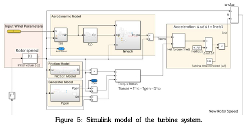
Wind Turbine Model

The major components of the wind turbine model are the electrical model of the generator, the mechanical model of the generator, bearings and the blades.

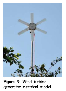
Note that the tail and yaw response has not been modelled. Hence this work assumes that the wind turbine is facing the wind at all times. The wind turbine used as the basis for the comparison in this paper is the Rutland 910 (Figure 1). The particular generator (Figure 2) does not produce a perfect sinusoidal voltage waveform, but the waveform has a significant 3rd harmonic component.

 

 

 

 

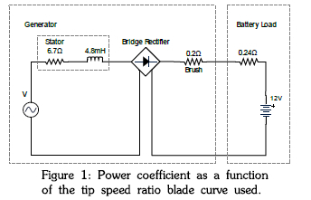
However, the rms voltage has been reasonably approximated as

V = 0.642w+ 0.4 (Equation 1)

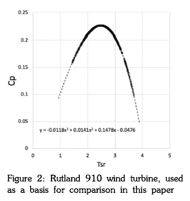
where w= rotor speed (radians per second) The blade model (Hossein, 1999) is a power coefficient versus tip speed ratio curve (Figure 3) that gives close results to the simulated turbine performance (Figure 4).

 

 

 

 

The mechanical parameters used are (Hossein, 1999):

D = 0.002 + O.OOle^-w)28 (Equation 2)

where D is the friction coefficient and the Moment of inertia, J = 0.1717 kgm².

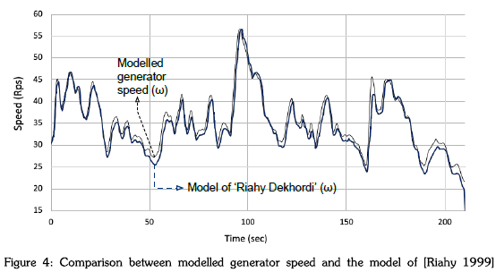
The blade Cp-Tsr curve was developed (Figure 3) and then, using the developed Simulink model of Figure 5, found to compare well (Figure 4) to the model of (Hossein, 1999). The rotor speed is used to validate the model because if the rotor speed is correct, then the output of the generator is also correct.

 

 

Output Power as a Function of Wind Speed

If instantaneous measurements of the wind speed and wind turbine output power are taken of this low inertia turbine at a turbulent wind site every 50ms for 3600s (one hour), a plot can be made of the output power versus the wind speed using the simulation model (Figure 6).

 

 

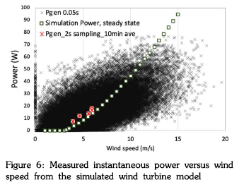
Figure 6 shows that there is a huge range of output powers for the same wind speed with the 50ms sampling. This results from that the turbine is either accelerating or decelerating while the simulation is running.

It is clear that the steady state power curve does not represent the average of the instantaneous readings. No sensible wind turbine power curve can be derived directly from this data.

If the IEC standard is used to determine the wind turbine performance, it involves sampling at least every 2-seconds and averaging over 10-minutes. Due to the limited extent of the data available to the authors, only six points could be plotted (Figure 6). However, the variation is also large enough not to be able to derive any power curve with any conviction. This indicates the difficulty of modelling low inertia wind turbines from sampled real time data in naturally gust wind conditions. Because of this difficulty, it is also difficult to accurately predict the energy production for a given wind speed regime. The next section examines the issues related to being able to reasonably predict the energy output of a wind turbine by using the simulation model of a wind turbine and sampled data.

 

Different Sampling Frequencies for Wind Speeds with 50ms Time Step Simulation

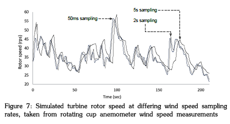
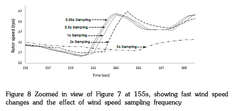
In Figure 7, for clarity, only rotor speeds calculated from three wind speed sampling times are shown, The 2-seconds sampling results are close to the 50ms sampling results. However, the 5-seconds sampling results are quite different, with phase delays and changes in the width of wind speed peaks. A closer examination of one of the peaks of Figure 7 is seen in Figure 8. Here, the 5-seconds sampling shows a potential issue in that the delay is long enough, such that if the wind speed had dropped as fast as it rose, the turbine speed would show a significant error. The conclusion is that when predicting the rotor speed, if the wind speed peak, or trough, is at a time scale less than that of the sampling rime, then for a wind turbine capable of reacting to the wind speed peaks and troughs, the simulated rotor speed, and hence power output of the turbine, will be incorrect. Hence the wind speed sampling time needs to be small compared to any rise or fall time of the wind speeds. The sampling time should also be small compared to any rise or fall in the speed of the wind turbine.

 

 

 

 

Energy Estimation using the direct method and method of bins

The energy is calculated using two methods. One method is using the power output from the wind turbine model in Simulink at different sampling interval to calculate the energy output. This method is referred to as the direct method in this analysis. The other method is the method of bins, as mentioned in the IEC standard (IEC Standard 614002, 2006). As per the standard, the wind speed should be sampled at a rate of 0.5Hz which is used to determine a 10-minute average. The wind speed data should then be binned into 0.5m/s wide wind speed bins. It should also be noted that IEC standard for data collection in the field is a very different scenario compared to investigating in a simulation environment. It is important to distinguish this point because IEC method samples both wind speed from the anemometer and power output from the wind turbine separately, specially for turbine testing. So, the power curve is the result of the measurements which are sampled and averaged separately. Whereas investigating the effect of different sampling times in simulation can be different from the investigation in the actual test site. Power output can vary depending on the type of data available and how its fed to the turbine model. This is discussed in detail in Figure 9.

The effect of wind speed sampled at different sampling and averaging periods on energy calculation has been analysed. A wind speed of 50ms raw data was available which was resampled to different lower frequencies for analysis. Figure 9, with four different figures, demonstrates the difference through diagrams and plots.

Figure 9-A is a typical IEC standard test station where different meteorological and wind turbine data is collected through different sensors and logged via a data acquisition system. In a Simulink environment illustrated by Figure 9-B, the wind turbine model produces power output at every timestep in accordance with the type of wind data available. Wind speed data sampled at different frequencies will produce different power outputs. The wind data resolution of the available wind speed and the simulation time step will determine how continuous the wind data is. As the sampling interval increases, the data becomes more discrete. For the wind turbine model, the turbine time constant must be the same as the simulation time step, the validity of which is already demonstrated in Figure 4. It is better to use a small timestep to generate continuous wind turbine output. However, the timestep also depends on the frequency at which the wind speed is sampled. If the timestep is less than the wind speed sampling interval, Simulink, in its default state, will linearly interpolate values between each data point. Timestep higher than the windspeed sampling interval will miss the actual data.

The Simulink analysis discussed in this investigation uses a 50ms timestep as this was the minimum sampling interval that could be set in the wind sensor.

Figure 9-C and figure 9-D are the zoomed in versions of one hour length of power plot for a better view. These figures intend to show power variation with the wind speed data available.

The output power from the wind turbine model indicated as 1 in Figure 9-B is graphically represented in figure 9-C with the same number and so on for the other outputs. The output power 1 is due to wind speed input sampled at 50ms. In this scenario, the wind speed input (50ms sampling) and the turbine model output (output 1) can be regarded as continuous output within the simulation environment. Output power 2 is the resampled power from output 1 and is what the IEC standard sampling will look like. In regard to power output 3, the wind turbine model receives a different wind speed resampled at 2-seconds with a sample and hold approach. Output 3 has a different shape than the rest of the power plot, as seen in Figure 9-C. The different shape is because of the windspeed resampling, which holds the sample until every next 2-seconds. The constant wind speed between intervals causes the turbine to accelerate, resulting in a sharp rise and fall of wind turbine speed and power. The power output 4 from the model occurs when the input wind data carries 2-seconds samples but is different in that no value exists between two intervals, unlike the earlier resampling approach using sample and hold. For power output 4, as the timestep is still 50ms, Simulink will now perform linear interpolation, which is why the power output 4 in Figure 9-D looks smoother than power output 3. The power variation in each of the mentioned cases grows in shape and magnitude compared to 50ms data as the sampling frequency increases. To investigate the effects of different sampling times in Simulink, 50ms sampled wind data adequately represents the actual dynamically changing wind speed. In Simulink, therefore, it is important to note the difference in power output and calculated energy not just as the sampling interval varies but also in how the resampling is implemented and what kind of data is fed into the model.

 

Energy calculation using the direct method

The wind speeds in Figure 10-A were measured with an ultrasonic anemometer with 50ms sampling in a turbulent wind area and are used as the basis for comparison. Due to the amount of data involved, the wind speed series consists of several combined from the same location to form a wind data of 60-minute span. The 50ms wind speed and power were resampled at 2-seconds intervals and averaged over 10-minute span to compare the energy estimation with the IEC recommendation. Both plot of wind speed and power in Figure 10A and Figure 10B clearly demonstrates the difference in IEC standard data and a 50ms raw data.

Figure 9-D demonstrated the power output 3 and power output 4 variations for approximately 35-seconds interval. But if the same two power output is averaged over 10-minute interval for a 60-minute data length, the variations are very small as can be seen in Figure 10-B.

The simulation time step has been kept constant at 50ms. In Figure 11-A, a vertical line separates the energy calculated with instantaneous samples and the average of 2-seconds samples. For Figure 11-A, the bars on the left (instantaneous sampling) are the total energy calculated using resampled wind speed output at various intervals fed to the wind turbine model separately. The power from the model is then used to calculate the energy for each sampling interval (e.g. power output 3 in Figure 9-B). The instantaneous energy seems to be less affected than the averaged energy. The most precise measure of the energy is at 50ms sampling, represented by the red bar in the far left of both bar plots of Figure 11.

The time plot of power gets significantly different in shape and values as the sampling frequency of wind speed changes, as demonstrated in section 4. However, it is notable that the sampling interval up to 30-seconds does not significantly change the total energy calculated using direct method for this example of wind speed. The average percentage difference of all energy calculated from 0.5-second to 30-second instantaneous sampling interval is less than 4%. However, as the averaging interval increases, the energy seems to increase as well as seen in Figure 11-A. The power from the wind turbine model is averaged over 10-minute interval of 2-second data. The 10-minute average overestimates the energy by 19%, whereas the energy at 1-minute interval is much closer to the energy calculated at 50ms. It is also important to note that the all averaged energy calculations are based on 2-seconds sampling interval. In a scenario, where only 10-minute data are available, and is fed to the wind turbine model, the energy decreases significantly by 45% for the 1 hour span of available wind data as shown in Figure 11-B. Figure 10-A shows the data vast difference in wind data resolution between 50ms and 10-minute averaged intervals which when passes through the wind turbine model results in significant variations in both for instantaneous power output and energy output as demonstrated by graphs (Figure 10-B and Figure 11).

 

Energy from Binned Wind Speeds

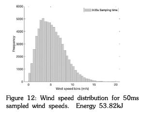
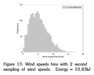
When the 50ms sampled wind data (Figure 10-A) from the one hour of wind data, is binned into 0.5m/s as per the standard, the results can be seen in Figure 12. If the wind speeds are sampled every 2-seconds, the distribution (Figure 13) is similar but has some notable differences in the bins of 3-5m/s and 10-11.5m/s.

 

 

 

 

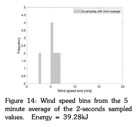
If now a 5-minute average is taken of the 2-seconds sampled data (Figure 14), a quite different wind speed distribution occurs. Although there is a shortage of time span for this approach, it illustrates an energy prediction issue.

 

 

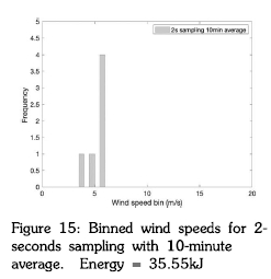
When the wind speeds are further averaged to 10-minute interval, it again results in very different wind distributions (Figure 15). If these distributions are used to estimate the wind turbine energy output from the wind turbine power curve, errors can be expected. However, for the present analysis, a steady state power curve is derived (Equation 3) using the wind turbine model at different constant wind speeds.

 

 

P = 0.59V² - 1.58V- + 0.1813 (Equation 3)

In this example, the energy predicted from the 50ms and 2-seconds sampled wind data bins is very similar at about 54kJ, but once the wind speeds are averaged, the calculated energy drops to about 37kJ. However, the energy calculated directly from the 50ms sampled wind data gives an energy level of 43.5lkJ. Hence the bins either overestimate the energy by 19% for instantaneous sampling or underestimate it by 11% and 22% in case for 5 minutes and 10-minutes averaging interval.

With much more data, such as over a year, it is possible that a more representative wind speed distribution will occur even for 10-minute averaged data. That may be good for grid feeding systems with constant tariffs, but for variable tariff systems, or for off grid systems, the amount of energy expected to be delivered on an hourly or daily basis is important as this will determine how much energy may be used and how much battery storage is required.

 

Conclusion

For the situation where the wind turbine can be expected to closely follow the changes in wind direction, a simulation investigation has been undertaken with measured wind speeds to determine the effect on the calculated energy output of the turbine, with different sampling intervals and averaging of the wind data. The energy at different sampling intervals was calculated directly using the model wind turbine and the method of bins. For the wind speed data used, the effect of sampling time from 50ms up to 20-seconds on the energy output calculated through the direct method was not significant. Although, the shape and magnitude of the wind speed start to change as the sampling interval increases beyond 2-seconds. The lower sampling time might be important for studies involving turbulence and structural fatigue. However, if the samples are averaged, a considerable difference in energy can occur. For the wind data used for the example, an overestimate of the energy of 19% is observed for data averaged at 10-minute intervals. From the investigation, it was also observed that in case where only 10-minute interval of wind data were only available, the energy overestimation would reach a drastic value of 42%.

Dividing wind data into bins to calculate the energy production from the wind turbine power curve showed that averaged sampled wind speeds underestimated the energy by 22%. At the same time, an overestimation of 19% was observed even at a lower sampling interval.

Overall, the result suggests that it might be better for this turbine to use sampled wind data at 2-seconds, without binning, than to bin or average the data. However, energy calculated directly using 1-minute average of 2-second sampled data produced only a 2% error. Therefore, 1 minute average could also be used considering long term data collection if both precision and volume of data are critical. Whilst long time period wind data (e.g. for one year) may alleviate the differences, small, off grid systems, with limited energy storage (e.g. in batteries), need to be able to accurately predict the energy production over a short period of time, such as an hour. Only then can the required energy storage be determined, as well as the number of days when there will not be enough energy. This requires a high sampling rate, higher than the fastest changes in the wind speed

 

References

Battisti, L. et al. (2018) Small Wind Turbine Effectiveness in the Urban Environment, Renewable Energy. Elsevier Ltd, 129, pp. 102113. doi: 10.1016/j.renene.2018.05.062.         [ Links ]

Doran, J. C. et al. (1977) Accuracy of Wind Power Estimates.         [ Links ]

Gross, M., Magar, V. and Pe a, A. (2020) The Effect of Averaging, Sampling, and Time Series Length on Wind Power Density Estimations, Sustainability, 12(8), p. 3431. doi: 10.3390/sul2083431.         [ Links ]

Hossein, G. (1999) Dynamic and Predictive Dynamic Wind Turbine Control. MONASH UNIVERSITY.         [ Links ]

IEC Standard 61400-2 (2006) International Standard - Part 2: Small Wind Turbines, 61010-1 n Iec:2001.         [ Links ]

Korprasertsak, N. and Leephakpreeda, T. (2018) Nyquist-Based Adaptive Sampling Rate for Wind Measurement Under Varying Wind Conditions, Renewable Energy. Elsevier Ltd, 119, pp. 290298. doi: 10.1016/j.renene.2017.12.018.         [ Links ]

Makkawi, A., Celik, A. and Muneer, T. (2009) Evaluation of Micro-Wind Turbine Aerodynamics, Wind Speed Sampling Interval and its Spatial Variation, Building Services Engineering Research and Technology, 30(1), pp. 714. doi: 10.1177/0143624408096343.e        [ Links ]

Rodriguez-Hernandez, O., del Ro, J. A. and Jaramillo, O. A. (2016) The Importance of Mean Time in Power Resource Assessment for Small Wind Turbine Applications, Energy for Sustainable Development. International Energy Initiative, 30, pp. 3238. doi: 10.1016/j.esd.2015.10.008.         [ Links ]

Roslan, E. et al. (2018) Effect of Averaging Period on Wind Resource Assessment for Wind Turbine Installation Project at UNITEN, in AIP Conference Proceedings, p. 020257. doi: 10.1063/1.5066898.         [ Links ]

Sunderland, K. et al. (2013) Small Wind Turbines in Turbulent (Urban) Environments: A Consideration of Normal and Weibull Distributions for Power Prediction, Journal of Wind Engineering and Industrial Aerodynamics. Elsevier, 121, pp. 7081. doi: 10.1016/j.jweia.2013.08.001.         [ Links ]

Tabrizi, A. B. et al. (2015) Rooftop Wind Monitoring Campaigns for Small Wind Turbine Applications: Effect of Sampling Rate and Averaging Period, Renewable Energy. Elsevier Ltd, 77, pp. 320330. doi: 10.1016/j.renene.2014.12.037        [ Links ]

 

 

* Corresponding author: Email: kimon.silwal@nmu.ac.za