ARTICLES
https://dx.doi.org/10.17159/2413-3051/2022/v33i1a7943

 

Using statistical tests to compare the coefficient of performance of air source heat pump water heaters

 

 

S. Tangwe^*; K. Kusakana

Department of Electrical, Electronic and Computer Engineering, Faculty of Engineering, Built Environment and Information Technology, Central University of Technology, Free State, South Africa

 

 

---

ABSTRACT

The study compared the coefficient of performance (COP) of two residential types of air source heat pump (ASHP) water heaters using statistical tests. The COPs were determined from the controlled volume of hot water (150, 50 and 100 L) drawn off from each tank at different time of use (morning, afternoon and evening) periods during summer and winter. Power meters, flow meters, and temperature sensors were installed on both types of ASHP water heater to measure the data needed to determine the COPs. The results showed that the mean COPs of the split and integrated type ASHP water heaters were 2.965 and 2.652 for summer and 2.657 and 2.202 for winter. In addition, the p-values of the groups COPs for the split and integrated type ASHP water heaters during winter and summer were 7.09 x 10^-24 and 1.01 x 10¹¹, based on the one-way ANOVA and the Kruskal-Wallis tests. It can be concluded that, despite the year-round performance of both the split and integrated type ASHP water heaters, there is a significant difference in COP at 1% significance level among the four groups. Furthermore, both statistical tests confirmed these outcomes in the comparisons of the mean COPs among the four groups based on the multiple comparison algorithm.
HIGHLIGHTS:
• One-way ANOVA multiple comparison test was used to verify any significant difference in the COPs among the four groups (classified by season and type of ASHP water heater).
• The Kruskal-Wallis multiple comparison test was used to see if any significant difference exists in the COPs among the four groups.
• The results demonstrated significant differences in the mean COPs amongst the four groups.
• The one-way ANOVA tests and the Kruskal-Wallis tests gave the same statistical outcomes.

Keywords: Air source heat pump water heater; p-value; significance level; one-way ANOVA test; Kruskal-Wallis test

---

 

 

1. Introduction

Hot water heating is responsible for a significant contribution to the electrical energy consumed in the residential sector, globally. In South Africa, 3050% of the electricity bill per month is from sanitary hot water production (Kivevele and Huan, 2014; Jaglin. and Dubresson, 2016). It has been observed that the majority of sanitary hot water production in the residential sector is achieved through the operation of inefficient electric geysers (Tangwe, 2018). Therefore, the necessity of an efficient mode of sanitary hot water heating becomes crucial. In addition, the electrical energy consumed by geysers through hot water heating can be reduced by 50-70% by retrofitting the existing geyser with an ASHP unit (Tangwe and Simon, 2019). ASHP water heaters are a renewable and efficient technology for sanitary hot water heating and are capable of utilising 1 unit of electrical energy to produce 3 or 4 units of useful output thermal energy to heat water to a set point temperature (Tangwe et al., 2014; Gang et al., 2011). The common types of residential ASHP water heaters in the South African markets are the split and integrated types (Harvey, 2012). The special characteristics associated with the excellent performance of the ASHP water heaters is called the coefficient of performance (COP) (Hepbasli and Kalinci, 2009). It must be emphasised that the COP of ASHP water heaters depends on the design of the components making up the closed loop circuit of the vapour compression refrigeration cycle, the ambient temperature, the volume of hot water consumption and the thermo-physical properties of the refrigerant (Ozgener and Hepbasli, 2005).

The ASHP water heaters can operate without the assistance of an auxiliary backup element under ambient temperature ranges from -4-40 ^oC (Morrison et al., 2004). The COP of an ASHP water heater is better during summer than winter, provided that the volume of hot water consumed is constant. Research conducted with identical split and integrated types of ASHP water heaters without auxiliary element showed that the integrated system performed better than the split type (Ibrahim et al., 2014). Indeed, limited studies have been conducted to test for any significant difference in COPs between two or more types of ASHP water heaters operating under the same conditions. Tangwe (2018) used the one-way analysis of variance (ANOVA) test to demonstrate that there exists a significant difference in the COPs of split and integrated type ASHP with an auxiliary heating element, operating under the same ambient conditions and with the same volume of hot water drawn off from each of the tanks. The use of statistical tests for comparing performance of a process or a quantity is only meaningful if the sample data is a true representation of the actual population and the data measurements were unbiased, with an acceptable uncertainty (Collins et al., 2001).

The study focused on the draw-off of controlled volumes of hot water from two identical split and integrated type ASHP water heaters: 150 L was drawn off in the morning (07:00-10:00); 50 L in the afternoon (13:00-15:00) and 100 L in the evening (17:00-20:00). The hot water set point temperature for each of the types of ASHP water heater was 55 ^oC. The systems were switched off before each specific volume of hot water was withdrawn and switched on simultaneously to allow for the systems to heat the stored water to its set point temperature. The simulated hot water draws mimic a typical hot water profile in South Africa for a high-or middle-income family of four, including two adults. The average COPs at the respective withdrawals of 150, 50 and 100 L, for each of the months of January to December 2018 were determined for the both types of ASHP water heaters. Furthermore, for each type, the determined COPs were divided into the summer months (January, February, March, April, September, October, November and December) and the winter months (May, June, July, August). The one-way ANOVA and the Kruskal-Wallis tests were used to show any significant difference in the COPs among the four groups (classified into the season and the type of ASHP water heater).

1.1 Terminology and calculation

1.1.1. One-way analysis of variance test

The one-way ANOVA test is used to verify if there exist any statistically significant differences between the means of more than two independent (unrelated) groups (Huberty and Morris, 1992; Johnson and Wichern, 2014). The ANOVA test has been recognised as the most common statistical method used in scientific and social research, and the main goal is to determine how much the groups in an experiment differ for the purpose of statistical significance (Laird and Mosteller, 1990; Breiman et al., 2017). Generally, if the confidence level for the one-way ANOVA test is assumed as 99%, then the significance level is 0.01 and the null hypothesis is rejected, when the p-value for the groups is less than or equal to 0.01. If the condition is fulfilled and the groups are normally distributed, then there exists a significant difference among the groups at 1% significance level. The p-value is determined from the probability of the F-statistic in the ANOVA table for the groups under consideration.

1.1.2. Kruskal-Wallis Test

The Kruskal-Wallis test is a nonparametric version of a classical one-way ANOVA test. It compares the medians of the groups of data to investigate whether the samples originate from the same population or equivalently, from different populations with the same distribution. The Kruskal-Wallis test uses ranks of the data, rather than numeric values, to compute the test statistics (TheodorssonNorheim, 1986). The F-statistics used in the classical one-way ANOVA test is replaced by a chi-square statistics and the p-value measures the significance of the chi-square statistics (Kulinskaya et al., 2003). In addition, the Kruskal-Wallis test assumes that all samples emanate from populations having the same continuous distribution, apart from possible different locations due to group effects, and that all observations are mutually independent (Kulinskaya et al., 2003). Similarly, if the confidence level for the Kruskal-Wallis test is assumed as 99%, then the null hypothesis is rejected if the p-value for the groups is less than or equal to 0.01. If the condition is fulfilled and the groups are continuous and from the same distribution, then there exists a significant difference among the groups at 1% significance level. The p-value is determined from the probability of the chi-statistics in the Kruskal-Wallis table for the groups under consideration.

1.1.3. COP of an ASHP water heater

It is the ratio of the useful thermal energy gained by the stored water and the input electrical energy consumed by the ASHP water heater during the vapour compression refrigeration cycle (Guo et al., 2011). The equation of the COP is given in Equation 1.

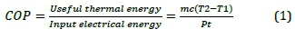
where m = mass of water heated by ASHP water heater and was measured by flow meter (F1); T2 = temperature of water exiting the outlet of the ASHP unit and was measured by the temperature sensor (T2); T1 = temperature of water entering the inlet of the ASHP unit and was measured by the temper ature sensor (T1); P = power consumed by the ASHP water heater and was measured by the power meters (P1 and P2); and t = time taken and was measured by the data logger (t); c = specific heat capacity of water (4.2 kJ/kg/k).

 

2. Materials and method

2.1 Materials

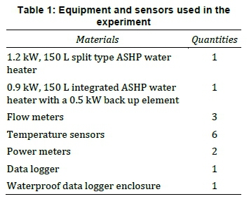
The list of equipment and sensors used in the setup is shown in Table 1.

 

 

2.2. Experimental setup

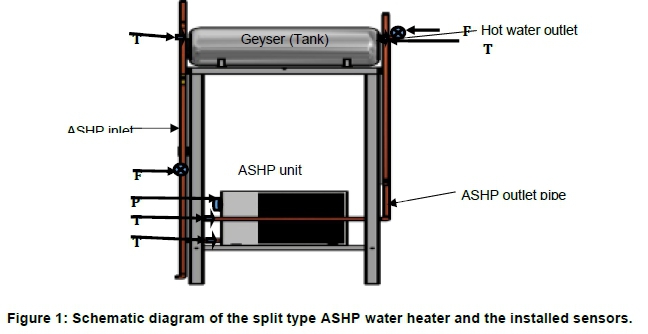
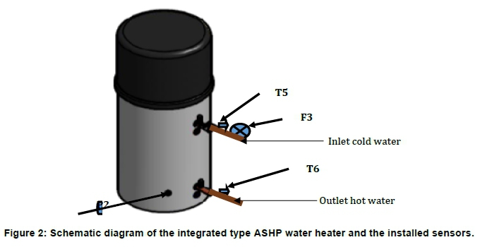
The study was conducted at the outdoor space of the renewable energy laboratory in the Yarona Building, Central University of Technology in the Free State province of South Africa. Figures 1 and 2 show schematic diagrams of the experimental setup. Flow meter F1 was installed in the proximity of the inlet pipe into the split type ASHP unit. Two flow meters (F2 and F3) were installed at the outlet pipes that allowed the hot water drawn off to exit the storage tanks of the split and integrated type ASHP water heaters. The temperature sensors T1 and T2 were installed at closed range on the pipes to the inlet and outlet of the split type ASHP unit. The temperature sensors T3 and T4 were installed on the pipes close to the inlet and outlet of the 150 L tank of the split type ASHP water heater. The temperature sensors T5 and T6 were installed on the pipes close to the inlet and outlet of the tank in the integrated type system. The power meters P1 and P2 were installed to measure the power consumed by the split and the integrated type ASHP water heaters, respectively. All the sensors were configured to log in five-minute interval throughout the monitoring period and were accommodated by a data logger. All the sensors and logger were products of Hobo Corporation and the configurations were done using the hoboware pro software.

 

3. Results and discussion

3.1. Summer operating performance of the split type ASHP water heater

150 L of hot water was drawn off in the morning (07:00-10:00), 50 L in the afternoon (13:0015:00), and 100 L in the evening (17:00-20:00), throughout summer, from both the split and integrated type ASHP water heaters. Both types were switched on simultaneously, after each controlled volume of hot water was drawn off. The COP for each type was determined for each specific hot water drawn off.

3.1.1. Summer COPs of the split type ASHP water heater

Table 2 shows the average COPs in each of the months in the summer season following the drawing off of 50, 100 and 150 L of hot water. It can be observed from Table 2 that during the 50 L hot water drawn off, the average time taken to heat the stored water to its set point temperature ranged from 35 to 40 minutes and the month-average duration was 38.5 minutes. The minimum and the maximum thermal energy gained was 2.19 and 2.44 kWh respectively, while the average was 2.33 kWh. The minimum and the maximum electrical power and energy consumed were 1.14 kW and 0.76 kWh, and 1.37 kW and 0.91 kWh respectively. The average-month power and the electrical energy consumed was 1.324 kW and 0.80 kWh. The COPs ranged from 2.70 to 3.04 and the average-month COP was 2.91.

 

 

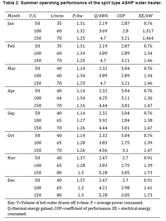
As displayed in Table 2, during the 100 L hot water drawn off, the average time taken to heat the water to its set point temperature ranged from 60 to 65 minutes and the average month time used was 63.0 minutes. The minimum and maximum thermal energy gained was 3.69 and 4.25 kWh respectively, while the average was 3.94 kWh. The minimum electrical power and energy consumed was 1.27 kW and 1.32 kWh, and 1.34 kW and 1.41 kWh respectively. The average-month power and electrical energy consumed was 1.31 kW and 1.37 kWh, respectively. The COPs were between 2.75 and 3.11 and the average was 2.88.

It is shown in Table 2 that during the 150 L hot water drawn off, the average month time taken to heat the water was 72.5 minutes. The average electrical power and the average electrical energy consumed as well as the average thermal energy gained was 1.27 kW, 1.53 kWh and 4.76 kWh respectively.

The COPs were between 3.01 and 3.21 and the average was 3.14.

3.1.2. Summer COPs of the integrated type ASHP water heater

Table 3 provides the average COP for the months in the summer season under the 50, 100 and 150 L of hot water drawn off. It shows that during the 50 L hot water drawn off, the average time taken to heat the water to its set point temperature was between 60 and 70 minutes and the average month duration was 63.75 minutes. The minimum and the maximum thermal energy gained was 2.19 and 2.47 kWh respectively, while the average was 2.33 kWh. The minimum and the maximum electrical power and electrical energy consumed were 0.85 kW and 0.86 kWh and 0.86 kW and 0.98 kWh respectively. The average month electrical power and electrical energy consumed was 0.85 kW and 0.90 kWh respectively. The COPs were between 2.50 and 2.70 and the average was 2.59.

It can be seen from Table 3 that during the 100 L hot water drawn off, the average time used to heat the water to its set point temperature was between 90 and 100 minutes and the average month time used was 95.0 minutes. The minimum and the maximum thermal energy gained was 3.69 and 4.25 kWh respectively, while the average was 3.88 kWh. The minimum and the maximum electrical power and energy consumed were 0.86 kW and 1.36 kWh, and 0.88 kW and 1.57 kWh, respectively. The average month electrical power and electrical energy consumed was 0.87 kW and 1.43 kWh respectively. The COPs were between 2.67 and 2.82 and the average was 2.72.

In accordance with the data presented in Table 3, the average month duration to heat the water was 125 minutes during the 150 L hot water drawn off. The average electrical power consumed, the average electrical energy consumed and the average thermal energy gained were 0.85 kW, 1.72 kWh and 4.58 kWh, respectively. The COPs ranged from 2.57 to 2.81 and the average was 2.65. Although the electrical power consumed by the integrated type was lower than for the split type under all the scenarios of hot water drawn off, the electrical energy consumed was higher while the COP was lower.

3.1.3. Winter COPs of the split type ASHP water heater

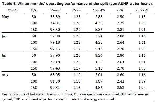
Table 4 shows the average COP per months in the winter season, for the 50, 100 and 150 L of hot water drawn off. With regards to the data displayed in Table 4, the average time used to heat the water to its set point temperature ranged from 55.39 to 63.05 minutes and the average month time was 58.56 minutes, during the 50 L hot water drawn off. The lowest and the highest thermal energy gained was 2.89 and 3.24 kWh respectively, while the average was 3.09 kWh. The fluctuation in electrical power and energy consumed was between 1.10 kW and 1.15 kWh, and 1.25 kW and 0.98 kWh, respectively. The average month power and electrical energy consumed was 0.85 kW and 1.16 kWh. The COP was between 2.50 and 2.80 and the average was 2.68.

It can be seen from Table 4 that during the 100 L hot water drawn off, the average time utilised to heat the water to its set point temperature was between 74.81 and 81.31 minutes and the average month time used was 78.62 minutes. The minimum and the maximum thermal energy gained was 3.86 and 4.39 kWh, while the average was 4.19 kWh. The minimum and the maximum electrical power and energy consumed were 1.18 kW and 1.60 kWh, and 1.28 kW and 1.61 kWh respectively. The average month power and the electrical energy consumed was 1.23 kW and 1.60 kWh. The COPs ranged from 2.42 to 2.75 and the average was 2.61.

Table 4 shows that during the 150 L hot water drawn off the average month duration to heat the water was 97.42 minutes. The average electrical power consumed, the electrical energy consumed, and the thermal energy gained were 1.18 kW, 1.91 kWh and 5.12 kWh respectively. The COPs varied between 2.53 and 2.81 and the average was 2.69.

3.1.4. Winter COPs of the integrated type ASHP water heater

Table 5 shows the average COPs for each month as a result of the 50, 100 and 150 L of hot water drawn off. It can be seen from Table 5 that during the 50 L hot water drawn off, the mean time used to heat water to its set point temperature varied between 74.85 and 79.86 minutes and the average month time was 77.81 minutes. The minimum and the maximum thermal energy gained was 2.89 and 3.24 kWh respectively, while the average was 3.09 kWh. The least and the greatest electrical power and energy consumed were 0.87 kW and 1.34 kWh, and 0.93 kW and 1.37 kWh respectively. The average month electrical power and energy consumed was 0.89 kW and 1.35 kWh respectively. The COP fluctuated between 2.10 and 2.42 and the average was 2.29. The average time taken to heat water to its set point temperature ranged from 105.42 to 112.58 minutes and the average was 110.01 minutes, during the 100 L hot water drawn off. The minimum and the maximum thermal energy gained were 3.87 and 4.39 kWh respectively, while the average was 4.19 kWh. The minimum and the maximum electrical power and energy consumed were 0.86 kW and 1.94 kWh, and 0.91 kW and 2.04 kWh, respectively. The average month power and electrical energy consumed were 0.89 kW and 1.97 kWh respectively. The COP ranged from 1.90 to 2.26 and the average was 2.14.

Table 5 shows that during the 150 L hot water drawn off, the average time to heat water to the set point temperature was 133.09 minutes. The average electrical power consumed, the electrical energy consumed and the thermal energy gained were 0.86 kW, 2.20 kWh and 5.13 kWh, respectively. The COPs varied between 2.05 and 2.29 and the average was 2.20. The electrical power consumed by the integrated type was lower than the split type under all the scenarios of hot water drawn off, but the electrical energy consumed was lower, while the COP was higher in the split type.

3.2. Comparison of the COPs among the four groups

The COPs of the ASHP water heaters were basically classified into four groups (the COPs during summer of the split type ASHP (COP_SS), the COPs dur ing summer of the integrated type ASHP (COP_SI), the COPs during winter of the split type ASHP (COP_WS) and the COPs during winter of the integrated type ASHP (COP_WI). The one-way ANOVA and the Kruskal-Wallis tests were used to investigate if any significant difference exists among the four groups at 99% confidence level and 1% significance level.

3.2.1. Comparison of the COPs among the four groups using the one-way ANOVA

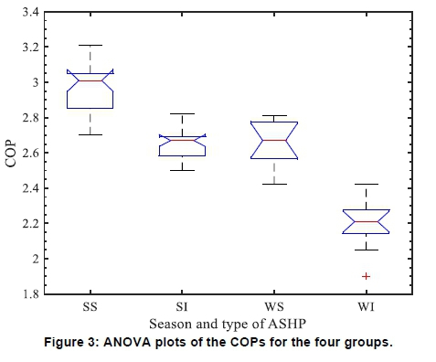
The data of the COPs among the four groups (COP_SS, COP_SI, COP_WS and COP_WI) were obtained from Tables 2, 3, 4 and 5. The four groups were classified such that a group of the COPs comprised both the season and the type of ASHP water heater. Hence, Figure 3 shows the one-way ANOVA plots of the four groups. The distribution among the four groups was normally distributed as there are negligible outliers shown in the Figure 3. The mean COP of the four groups (COP_SS, COP_SI, COP_ WS and COP_WI) was 2.965, 2.653, 2.658 and 2.205 respectively. The mean COP of the group COP_SS was the highest, while the mean COP of the group COP_WI was the lowest, as shown in the red line on each of the group's in the ANOVA plots. The upper and lower horizontal black lines on each of the ANOVA plots represent the upper and lower limits of the COPs for each group. Table 6 shows the oneway ANOVA table from the distribution of the four groups. It can be seen that the sum of squares between the four groups was 4.679, while the sum of squares within the groups was 1.154. The mean square between the groups is the ratio of the sum of squares between the groups and the degree of freedom between the groups is 4.679/3 = 1.56. The mean square within the groups is the ratio of the sum of squares within the groups and the degree of freedom within the groups is 1.154/68 = 0.017. The F-statistics is the ratio of the mean square between the groups and the mean square within the groups is 1.56/0.017 = 91.9. The probability of the F-statis-tics gives the p-value. The p-value of the four groups was 7.0 x 10^-24, much smaller than 0.01. Hence, the null hypothesis that there is no mean significant difference among the four groups of COPs is rejected. Therefore, there exists a significant difference of the COPs among the four groups at 1% significance level.

 

 

3.2.2. Using the ANOVA-multiple comparison algorithm to compare the four COPs groups

The ANOVA-multiple comparison test used the statistics from the one-way ANOVA test to perform a test which verified if any significant difference exists between all possible pairs of groups among the original groups. The differences in the true means at the lower and upper 99% confidence level between pairs of groups among the four groups were determined. If the difference in the true means of the lower confidence level and the difference in the true means of the upper confidence level of the pairs of groups was such that the range of the interval included 0, there is no significant difference between the pairs of groups. On the contrary, if the difference in the true means at the lower confidence level and the difference in the true means at the upper confidence level of the groups' pairs was such that, the range between the two confidence levels do not included 0, a significant difference exists between the groups' pairs.

Table 7 shows the ANOVA-multiple comparison table generated from the statistics obtained from the four groups of COPs. It shows that five of the six groups' pairs derived from the four groups showed a significant difference in the COPs. The comparison between the pair of groups COP_SI and COP_WS showed no significant difference at the 1% significance level, as the difference between the pair of the true mean COPs at the lower confidence level (0.1259) and that at the upper confidence level (0.1167) recorded 0, in the range of the confidence interval. However, the p-value between the groups pair of COP_SI and COP_WS was 0.9996, thus greater than 0.01. It can be seen that the p-values between the rest of the five groups' pairs showed significant differences at the 1% significance level, as the p-values were less than 0.01 and their confidence interval ranges did not include 0.

3.2.3. Comparison of the COPs among the four groups using the Kruskal-Wallis test

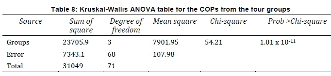
The data of the four groups (COP_SS, COP_SI, COP_WS and COP_WI) were obtained from Tables 2, 3, 4 and 5. The mean ranks of the group's COPs of the four groups were 58.910, 31.060, 32.450 and 6.580 respectively. Table 8 shows the Kruskal-Wallis table for the distribution derived from the four groups. The Kruskal-Wallis table is similar to the one-way ANOVA table except that the analysis was performed with the mean ranks of the distribution and not the mean values. In addition, the F statistics in the one-way ANOVA test are replaced by the chi-statistics in the Kruskal-Wallis ANOVA table.

It can be observed from Table 8 that the sum of squares between the four groups in terms of mean ranks was 23705.9, while the sum of squares within the groups was 7343.1. The chi-square is the ratio of the mean square between the groups and the mean square within the groups (7901.95/107.99 = 54.21). The probability of the chi-square gives the p-value. The p-value was 1.01 x 10^-11, much smaller than 0.01 significance level. Hence, the null hypothesis, indicating that there is no significant difference among the groups COPs, is rejected. Therefore there is a significant difference of the COPs among the four groups at 1% significance level.

3.2.4. Using the Kruskal Wallis-multiple comparison algorithm to compared the four COP groups

The Kruskal-Wallis-multiple comparison test employed the statistics from the one-way ANOVA, however, in terms of mean ranks to perform the test, which investigated whether any significant difference exists among three or more groups by testing for significant difference between groups pairs among the original groups. This was achieved by computing the true mean ranks of the lower and upper 99% confidence level of each of the groups, and then subtracting the corresponding true mean ranks of the lower and upper 99% confidence level for each between groups pairs among the original groups. If the difference in the true mean ranks of the lower confidence level and the difference in the true mean ranks of the upper confidence level of the between groups' pairs were such that the range of the interval included 0, there exists no significant difference between the groups pairs. The p-values between the group pairs could not be used solely, as the interval range comparison does not occur simultaneously. Table 9 shows the Kruskal-Wallis- multiple comparison table generated from the statistics obtained from the four groups using the mean ranks COPs.

Table 9 shows that five of the six pairs of the between groups show a significant difference among the four groups of COPs. The comparison between groups' pair of the groups COP_SI and COP_WS showed no significant difference of the COPs at 1% significance level. This indicated that the difference between the pair of the true mean rank COPs at the lower confidence level (-20.39) and at the upper confidence level (17.5982), was 0 - in the confidence interval range. However, the p-value between the groups' pair mean rank COPs (COP_SI and COP_WS) was 0.9976 and was greater than 0.01.

 

4. Conclusion

It can be concluded without the loss of generality that among the four groups, the average COPs of the group COP_SS were the best, followed by the groups COP_SI, COP_WS and COP_WI, from a basic analytical approach. It can be demonstrated that the average electrical energies consumed by the split type

ASHP water heater during summer was the least, while the average electrical energies consumed by the integrated type ASHP water heater was the greatest. Based on the determination of averages from the analytical perspective, it is not possible to justify if there is any significant difference among the four groups of COPs. Application of the one-way ANOVA and the Kruskal-Wallis tests allowed a determination as to whether there is any mean significant difference among the four groups COP_SI, COP_WS and COP_WI. Both the one-way ANOVA and Kruskal-Wallis tests showed that there is a significant difference at the 1% significance level among the four groups. Furthermore, the ANOVA-multiple comparison tests and the Kruskal-Wallis -multiple comparison tests were used for the COPs groups to show that there exists a significant difference between five of the six groups' pairs (these include the following COPs groups' paired: COP_SS and COP_SI; COP_SS and COP_WS; COP_SS and COP_WI; COP_SI and COP_WI; and COP_WS and COP_WI) among the four groups. However, it must be noted that the multiple comparison test using the Kruskal-Wallis test is not a simultaneous comparison tests, and in some scenarios the outcome from the range of the confidence interval test might differ from the results of the p-value. Hence, in cases wherein the confidence interval result disagreed with the p-value through the Kruskal-Wallis-multiple comparison test, the correct and acceptable result is obtained from the range of the confidence interval. It can also be concluded that throughout the operating scenarios the backup heating element of the integrated type ASHP water heater did not switch on. Finally, the two tests gave identical predictions on the verification of any significant difference between all the groups' paired among the four groups, without any discrepancy.

 

Acknowledgement

The authors acknowledge the Central University of Technology, in Free State, South Africa for financial support to ward the acquisition of the research equipment.

 

Author contributions

S. Tangwe: Conceptualisation, drafting and development of the manuscript.

K. Kusakana: Technical input, technical restructuring and proofreading of the manuscript.

 

References

Breiman, L., Friedman, J.H., Olshen, R.A. and Stone, C.J., 2017. Classification and regression trees. Routledge.         [ Links ]

Collins, L.M., Schafer, J.L. and Kam, C.M., 2001. A comparison of inclusive and restrictive strategies in modern missing data procedures. Psychological Methods, 6(4): 330.         [ Links ]

Gang, P., Guiqiang, L. and Jie, J., 2011. Comparative study of air-source heat pump water heater systems using the instantaneous heating and cyclic heating modes. Applied Thermal Engineering, 31(2-3): 342-347.         [ Links ]

Guo, J.J., Wu, J.Y., Wang, R.Z. and Li, S., 2011. Experimental research and operation optimization of an air-source heat pump water heater. Applied Energy, 88(11): 4128-4138.         [ Links ]

Harvey, L.D., 2012. A handbook on low-energy buildings and district-energy systems: Fundamentals, techniques and examples. Routledge.         [ Links ]

Hepbasli, A. and Kalinci, Y., 2009. A review of heat pump water heating systems. Renewable and Sustainable Energy Reviews, 13(6-7): 1211-1229.         [ Links ]

Huberty, C.J. and Morris, J.D., 1992. Multivariate analysis versus multiple univariate analyses. In Kazdinm A.E. (Ed.), Methodological Issues and Strategies in Clinical Research: 351-365. American Psychological Association. https://doi.org/10.1037/10109-030        [ Links ]

Ibrahim, O., Fardoun, F., Younes, R. and Louahlia-Gualous, H., 2014. Review of water-heating systems: General selection approach based on energy and environmental aspects. Building and Environment, 72: 259-286.         [ Links ]

Jaglin, S. and Dubresson, A., 2016. Eskom: Electricity and technopolitics in South Africa. Juta.         [ Links ]

Johnson, R.A. and Wichern, D.W., 2014. Applied multivariate statistical analysis (Vol. 6). London, UK: Pearson.         [ Links ]

Kivevele, T. and Huan, Z., 2014. A review on opportunities for the development of heat pump drying systems in South Africa. South African Journal of Science, 110(5-6): 01-11.         [ Links ]

Kulinskaya, E., Staudte, R.G. and Gao, H., 2003. Power approximations in testing for unequal means in a one-way ANOVA weighted for unequal variances. Communications in Statistics-Theory and Methods, 32(12): 2353-2371.         [ Links ]

Laird, N.M. and Mosteller, F., 1990. Some statistical methods for combining experimental results. International Journal of Technology Assessment in Health Care, 6(1): 5-30.         [ Links ]

Morrison, G.L., Anderson, T. and Behnia, M., 2004. Seasonal performance rating of heat pump water heaters. Solar Energy, 76(1-3): 147-152.         [ Links ]

Ozgener, O. and Hepbasli, A., 2005. Experimental performance analysis of a solar assisted ground-source heat pump greenhouse heating system. Energy and Buildings, 37(1): 101-110.         [ Links ]

Tangwe, S., Simon, M. and Meyer, E., 2014. Mathematical modeling and simulation application to visualize the performance of retrofit heat pump water heater under first hour heating rating. Renewable Energy, 72: 203-211.         [ Links ]

Tangwe, S.L., 2018. Demonstration of residential air source heat pump water heaters performance in South Africa: Systems monitoring and modelling. Doctoral dissertation, University of Sunderland.         [ Links ]

Tangwe, S.L. and Simon, M., 2019. Quantification of the viability of residential air source heat pump water heaters as potential replacement for geysers in South Africa. Journal of Engineering, Design and Technology, 17(2): 456-470.         [ Links ]

Theodorsson-Norheim, E., 1986. Kruskal-Wallis test: BASIC computer program to perform nonparametric one-way analysis of variance and multiple comparisons on ranks of several independent samples. Computer Methods and Programs in Biomedicine, 23(1): 57-62.         [ Links ]

 

 

* Corresponding author: Email: lstephen@cut.ac.za