ARTICLES

 

Offshore wind energy - South Africa's untapped resource

 

 

Gordon Rae^{I. *}; Gareth Erfort^II

^IDepartment of Mechanical and Mechatronic Engineering, Stellenbosch University, Stellenbosch 7599, South Africa. ORCiD 0000-0002-6848-0173
^IIDepartment of Mechanical and Mechatronic Engineering, Stellenbosch University, Stellenbosch 7599, South Africa. ORCiD 0000-0001-7986-1281

 

 

---

ABSTRACT

In the context of the Anthropocene, the decoupling of carbon emissions from electricity generation is critical. South Africa has an ageing coal power fleet, which will gradually be decommissioned over the next 30 years. This creates substantial opportunity for a just transition towards a future energy mix with a high renewable energy penetration. Offshore wind technology is a clean electricity generation alternative that presents great power security and decarbonisation opportunity for South Africa. This study estimated the offshore wind energy resource available within South Africa's exclusive economic zone (EEZ), using a geographic information system methodology. The available resource was estimated under four developmental scenarios. This study revealed that South Africa has an annual offshore wind energy production potential of44.52 TWh at ocean depths of less than 50 m (Scenario 1) and 2 387.08 TWh at depths less than 1 000 m (Scenario 2). Furthermore, a GIS-based multi-criteria evaluation was conducted to determine the most suitable locations for offshore wind farm development within the South African EEZ. The following suitable offshore wind development regions were identified: Richards Bay, KwaDukuza, Durban, and Struis Bay. Based on South Africa's annual electricity consumption of297.8 TWh in 2018, OWE could theoretically supply approximately 15% and 800% of South Africa's annual electricity demand with offshore wind development Scenario 1 and 2 respectively.

Keywords: renewable energy; resource assessment; site selection; offshore wind energy potential; GIS spatial analysis

---

 

 

1. Introduction

The International Energy Agency (IEA, 2016) predicts that global electricity demand will increase by approximately 56% by 2050. Empirical data highlights that electricity generation contributes to more than 40% of global energy-related CO2 emissions (Ang & Su, 2016). To prevent negative irreversible environmental impact, it was agreed on at the 2015 Paris Climate Conference (COP 21) to limit global temperature increases to below 1.5 °C above preindustrial levels (UNFCCC, 2015). It has been estimated that in order to guarantee a 50% probability of global temperatures remaining below the 2 °C limit, global CO2 emissions must remain below 1440 gigatons between 2000 and 2050 (McGlade & Ekins 2015). Achieving the goal of emitting less than 1 440 gigatons of CO2 by 2050 will not be possible without the partial or full decoupling of CO2 emission from electricity generation (Meinshausen et al., 2009).

During the COP21, South Africa was one of many nations that signed an intended nationally determined contribution (INDC) to commit to reducing carbon emissions. South Africa has pledged to decrease carbon emissions by a significant 42% by 2025 (Fakir, 2015). According to the Department of Environmental Affairs (DEA, 2015), reducing South Africa's dependence on coal-fired power generation and increasing its renewable energy (RE) fleet is the most logical and feasible means of South Africa achieving its decarbonisation goal.

The urgency for decarbonisation, coupled with both the price reduction and abundance of wind and solar resources in South Africa, makes investment in these technologies an obvious decarbonising strategy. South Africa currently has the Renewable Energy Independent Power Producer Procurement Programme (RE14P) in place for the procurement of RE projects. The REI4P successfully procured 6 400 MW of power in its first four bid windows (DOE, 2019), but is yet to exploit or consider the abundance of offshore wind energy (OWE) resources available to South Africa. This study quantifies these OWE resources, to inform key stakeholders of this significant untapped resource.

1.1 OWE resource assessment

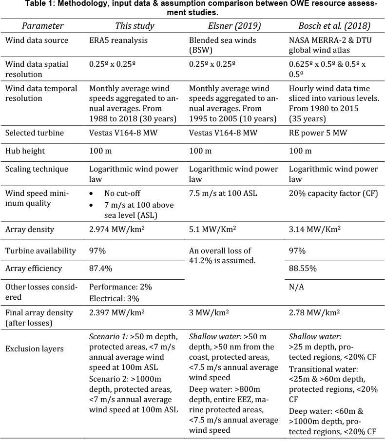
The increase in the number of earth observation satellites has stimulated the collection of global-scale atmospheric data (Bosch, Staffell & Hawkes, 2018). Globally, wind data is now available from either meteorological models or via satellite observation (Elsner, 2019). The increase in large atmospheric data has allowed for OWE resource assessment studies to be conducted using a bottom-up approach (Bosch et al., 2018; Dupont, Koppelaar & Jeanmart, 2018). Four average wind speed satellite observation datasets, which have been used in similar resource assessment studies, are compared in Table 1.

Offshore wind is a clean energy generation technology that holds significant resource potential to many coastal nations. Elsner (2019) conducted a continental-scale offshore wind resource assessment of Africa, his results showing a gross OWE resources capacity of26 968 GW. Hence, OWE has significant potential to play a pivotal role in Africa's large-scale energy-sector decarbonisation.

Recently, there has been emphasis within academia to quantify OWE resources (Bosch et al., 2018; Elsner, 2019; Musial, Heimiller, Beiter, Scott & Draxl, 2016). These referenced studies quantify OWE resources using similar methodologies on multiple scales, ranging from local to global. Table 1 offers an in-depth comparison of the methodologies, data inputs and assumptions of this study, against similar assessments. Bosch et al. (2018) and Elsner (2019), were selected as comparative studies as they both provide an offshore annual energy production (AEP) estimate for South Africa, allowing the direct comparison of methodologies and results. Elsner and Bosch et al. both indicate that South Africa has significant OWE resource potential. Bosch et al. calculated an AEP estimate for South Africa of 3100 TWh; Elsner arrived at a more conservative estimate of 2 821 TWh. The variation in results are derived from the methodology and data discrepancies highlighted in Table 1, but despite the difference, these studies both clearly highlight the significant potential for OWE development in South Africa.

1.2 Scope and limitations

OWE resource assessment studies are essential for the development of local offshore wind industries.

Quantifying the OWE resource is a fundamental first step for the development of OWE markets, and offers valuable insight for national-level energy system planning and private sector investment (Bosch et al., 2018). This study quantifies the OWE resource available to South Africa under four developmental scenarios, and identifies the most suitable wind farm development regions within the South African exclusive economic zone (EEZ) - the first study to do so. The study is further unique, as the first OWE resource assessment to focus exclusively on the South African context. The wind speed dataset used is the ERA5 climate reanalysis dataset. This presented some limitation, as this dataset has a resolution of 0.25° x 0.25°, which created small data gaps within the study area at points where the dataset met the study area borders, such as the EEZ and terrestrial boundaries. Furthermore, this study did not consider the effect of shipping lanes on resource potential and site selection.

 

2. Data inputs

2.1 Wind

The ERA5 climate reanalysis dataset is developed by the Copernicus Climate Change Service (C3S). Data processing for the ERA5 is carried out using ECMEFS' Earth System Model IFS (Hennermann, 2019). The reanalysis methodology combines satellite observations into globally complete fields. The native resolution of the ERA5 atmosphere and land reanalysis is 31 km on a reduced Gaussian grid. This reanalysis data has been re-gridded onto a regular lat-lon grid of 0.25° x 0.25°. The re-gridded resolution has an uncertainty estimate of between 0.5° and 1° (Hennermann, 2019). The ERA5 reanalysis provides data at a three-hour time resolution. To facilitate climatic operations, this data was been pre-calculated by C3S to display monthly averages.

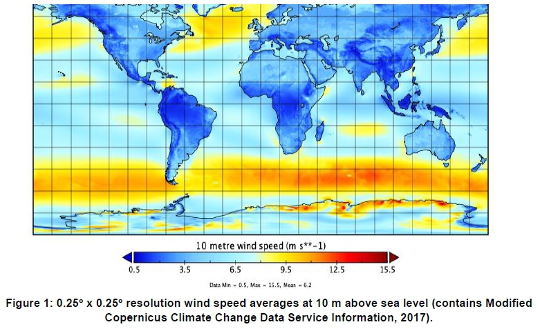
To accurately simulate a long-term wind resource, a 30-year time series of monthly average wind speeds from January 1988 to January 2018 was required as the raw wind speed dataset for this study (C3S, 2017). This raw dataset was subject to various forms of processing, including statistical averaging, boundary reduction, and vertical extra-po-lation. A data processing software called Climate Data Operator (CDO) was employed to calculate a single monthly wind speed average per raster pixel. A time average function on CDO was used to determine a statistical monthly wind speed average from the 30-years of monthly wind speed data, at a 0.25° x 0.25° pixel resolution. Figure 1 illustrates the average monthly wind speeds at 10 m above sea level (ASL), displayed on a 0.25° x 0.25° raster pixel resolution. Figure 1 was developed using a NetCDF graphical display application called Panoply.

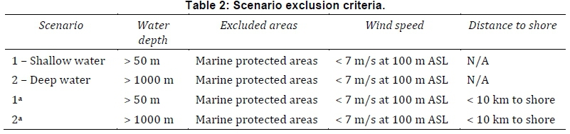
As shown in Table 2, a cut-off wind speed of 7 m/ s was introduced in this study, as, according to Musial et al. (2016), areas with wind speeds less than 7 m/s become economically unfeasible for offshore wind development.

2.2 Bathymetry

Ocean bathymetry data is critical to this study, as it allows for the determination of suitable offshore wind development regions. It would be inaccurate to assume the entire EEZ as the potential development area as there are certain OWE technology constraints.

The OWE industry has experienced significant technological advancements in terms of offshore wind turbine (OWT) foundations. The development of floating OWT foundations allow OWTs to be commissioned at significant depths. Previous OWE resource assessment studies have used an ocean depth upper limit of 800-1 000 m when defining their development scenarios (Bosch et al., 2018; Elsner, 2019; Musial et al., 2016). The industry upper limit for feasible deployment depths has been set at 1 000 m (Musial et al., 2016). This depth has been accepted as a rational upper operational limit after the Hywind floating wind farm was constructed at a depth of 800 m (Equinor, 2017).

The ocean bathymetry data for this study was sourced from the General Bathymetric Chart of the Oceans (GEBCO). This study uses the GEBCO_2014 dataset, which has a spatial resolution of 30 arc seconds - this was the most up-to-date and accurate ocean bathymetry dataset available.

2.3 EEZ and marine protected regions

This study uses global EEZ data accessed from Flanders Marine Institute (2014) data depository. As previously mentioned, the entire EEZ is not feasible for OWE generation, due to bathymetry and to land-use restrictions including marine protected areas, such as national parks and heritage sites. Such regions are removed from the study area and their respective OWE generation potentials are not included in the final AEP estimations. The protected region data was sourced from the World Database on Protected Areas, the most comprehensive database on terrestrial and marine protected areas (UNEP-WCMC, 2019).

2.4 Scenario modelling

Four unique development scenarios were created to assess the OWE resource potential available to South Africa. These scenarios have unique developmental regions which were defined by the spatial constraints listed in Table 2. The methodology of creating developmental scenarios has been used in a wide range of OWE resource assessment literature (Bosch et al., 2018; Dupont et al., 2018; Elsner, 2019; Hong & Möller, 2011; Musial et al., 2016). This study explores two primary developmental scenarios, namely, Scenarios 1 and 2, for deep water and shallow water analysis. These scenarios are modelled in order to quantify the OWE resource potential available to fixed bottom and floating OWT technologies respectively.

Mature European OWE markets have implemented policy that keeps OWE development out of a 10 km buffer from the coastline (Bosch et al., 2018), to prevent undesirable visual impacts which can negatively affect tourism, natural aesthetics and the value of coastal real estate. This study adopts a similar approach to that made by Bosch et al. (2018) to model the effects of restrictive policy. This study creates a developmental restrictive buffer area that extends 10 km orthogonally from the coastline, removing the generation potential within this buffer from the final AEP estimations. By doing so, this study quantifies the effect that developmental restrictive policy will have on the OWE resource potential available to South Africa, as it is likely that the future South African OWE industry will implement policy similar to that of mature industries. Scenarios 1^a and 2^a, derivatives of Scenario 1 and 2, were created to account for the visual impacts created by offshore wind farms. Table 2 gives details of the four developmental scenarios used in this study, showing the exclusion criteria used.

 

3. Methodology

3.1 Overview

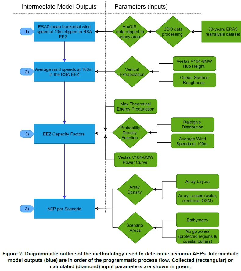
The methodology adopted for this study is a bottom-up approach, which has been broadly accepted and exercised in this field of academia (Bosch et al., 2018; Dupont et al., 2018; Elsner, 2019). The bottom-up approach calculates the CF per raster pixel using spatially accurate wind speed data and turbine specifications. A diagrammatic outline of the methodology used to calculate the various scenario AEPs is given in Figure 2.

The Vestas V164 - 8 MW turbine was selected for this study because, firstly, at the time of the study it represented the current state of art offshore turbine technology; secondly, for supply chain reasons - Vestas already has a large footprint in the South African wind energy industry.

The ERA5 wind data was vertically extrapolated to the Vestas V164 - 8 MW hub height of 100 m, using the logarithmic profile law. To account for the annual distribution of wind speeds, Rayleigh's frequency distribution was assumed and applied to the spatially accurate average wind speed raster file.

Once average wind speeds and annual distributions were determined at a pixel resolution, power outputs per average wind speed were calculated using the Vestas V164 - 8 MW power curve. The capacity factor is the ratio of actual annual turbine power output to the annual rated power output. Once the relationship between average wind speed and CF was determined, it was used in GIS to generate a new, spatially accurate CF raster file using the raster calculator tool.

To calculate the wind energy generation potential, a farm layout was assumed. From this, an array density in MW/km² was calculated. Losses, such as wake losses, electrical losses, and O&M losses, were all factored in during this step to determine a final turbine array density. The CF per pixel was multiplied by the array density to arrive at a wind energy generation potential per pixel. The estimated AEP of individual pixels within the South African EEZ were summed together to determine the final estimated AEP per scenario.

3.2 Wind data processing

The ERA5 dataset utilised up to this point of the study described wind speed data at 10 m ASL. It was necessary to height adjust these wind speeds to the V164 - 8 MW turbine hub height of 100 m. The wind speed height adjustment was achieved using the logarithmic wind profile law illustrated in Equation 1:

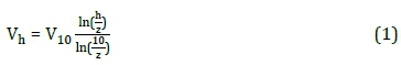
where V_h is the velocity of wind at the height of h; z is the surface roughness coefficient; and V₁₀ is the wind velocity at a height of 10 m.

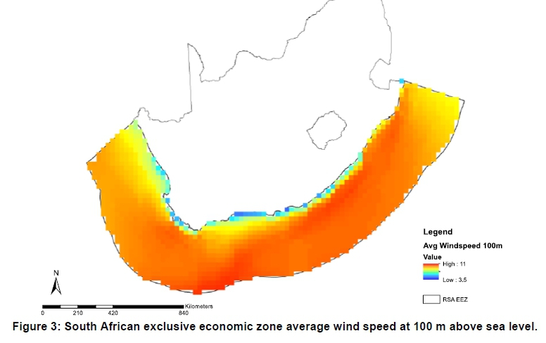
A standard value for ocean surface roughness of 2 e^-4 m was applied (Dvorak, Archer & Jacobson, 2010). This equation was used in the raster calculator tool on ArcGIS to create a new raster file that displayed wind speeds at 100 m ASL. Figure 3 shows the South African EEZ average wind speeds at 100 m ASL at a 0.25° x 0.25° spatial resolution.

The data created in this new shapefile was used in the next section to determine the relationship between capacity factor and average monthly wind at 100 m ASL.

3.3 Capacity factor

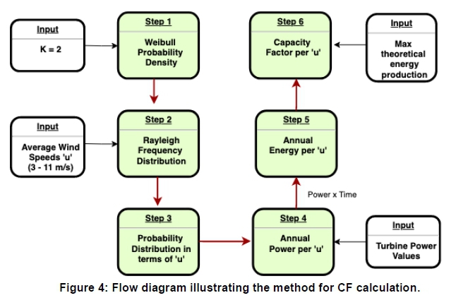
This section explains the methodology, inspired by Elsner (2019), that was used to determine the CF at each 0.25° x 0.25° raster pixel within the study area. Figure 4 illustrates the methodology. Further, the steps listed below offer a detailed breakdown of the methodology required to determine the CF per pixel resolution.

1. To calculate the CF, it was necessary to estimate the probability of occurrence f(v) of specific wind speeds V. This was achieved with the use of the Weibull probability density function, expressed in Equation 2:

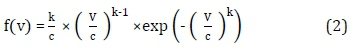
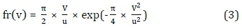
where c is the scale parameter in m/s, and k is the dimensionless form-parameter that specifies the shape of the Weibull distribution. A large value for k indicates constant winds and a low value represents variable winds (Elsner, 2019). As this study has a large area of interest, it was challenging to parameterise c and k values. It is commonly assumed that the shape factor has a value of k = 2, as this describes the frequency distribution relatively well (Elsner, 2019). Allowing k = 2 is an approach that has been used in a number of wind energy resource assessments conducted on large study areas (Andrews & Jelley 2007; Eisner, 2019; Yamaguchi & Ishihara 2014). According to Els-ner (2019), adopting a shape factor of k = 2 has the additional benefit of simplifying the Weibull distribution into a Rayleigh frequency distribution, which defines the probability distribution is terms of an average wind speed u. The Rayleigh distribution defines the frequency fr(v) of wind speed v occurring in a region experiencing average wind speed u. This is illustrated in Equation 3, where V² and u² are the square of the wind speed and average wind speed respectively.

As illustrated by Busby (2012), this equation can be modified to convert the frequency from a percentage of time to a number of hours per year, H, by multiplying the equation by 8 760. This is illustrated in Equation 4.

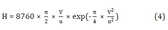
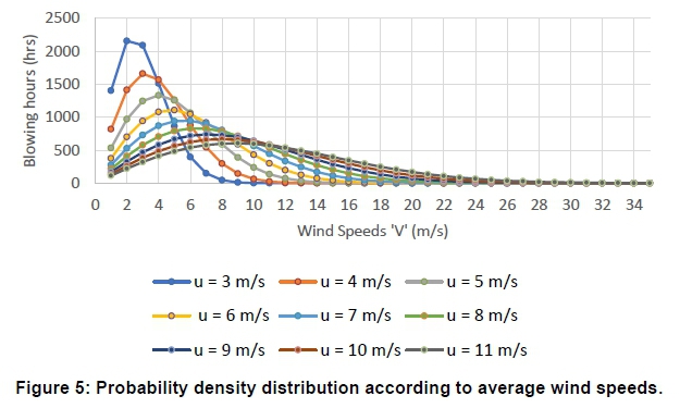
2. Next, Equation 4 was used in conjunction with the range of average wind speeds found within the South African EEZ at a height of 100 m ASL. The average wind speed range of the study area is 3-11 m/s (see Figure 2).

3. The output of Step 2 yielded a unique probability density distribution for each of the aforementioned average wind speeds (Figure 5).

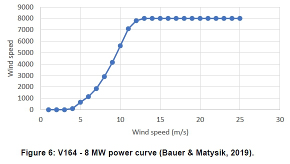
4. Next, the power at each wind speed was determined using the V164 - 8 MW power curve, which is illustrated in Figure 6.

 

 

5. After the power at each wind speed was quantified, the AEP at each wind speed was calculated by multiplying the power of each wind speed by the number of annual hours the respective wind speed was predicted to blow. After the power at each wind speed was quantified, the AEP at each wind speed was calculated by multiplying the power of each wind speed by the number of annual hours the respective wind speed was predicted to blow (this step yielded energy values in MWh). The AEP for each average wind speed was determined by summing the energy values of all the wind speeds V that existed in each average wind speed u (the range of wind speeds, V, that exist in each average wind speed, u, are shown in Figure 4). The full and detailed calculations can be found in Rae (2019).

6. The CF was calculated using Equation 5.

where E_gen is the total annual energy in MWh generated at each individual average wind speed; and E_rated is the theoretical maximum energy that the V164 - 8 MW turbine could produce in a year. As shown in the flow diagram, E_rated was required as an input for this step. The E_rated was calculated by multiplying the P_rated of the V164 - 8 MW by the number of hours in a given year. This assumes the turbine will be running at P_rated for 100% of the year.

The V164 - 8 MW has an E_rated of 70 080 MWh/year. The E_gen for each average wind speed is divided by the E_rated to determine a CF for each average wind speed. Figure 7 shows the relationship between the average wind speeds and their respective CFs.

A trend line was added to the graph in Figure 7 and a 4^th order polynomial relationship was generated to accurately depict the relationship between u and CF. This relationship is illustrated in Equation 6.

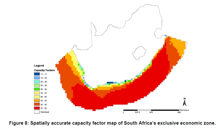
This relationship was applied to the previous spatially accurate average wind speed map of the study area at 100 m (Figure 2) and yielded a 0.25° x 0.25° resolution, spatially accurate CF map of the study area. This result is displayed in Figure 8.

3.4 Array density

This study assumed a 10 x 10 turbine array size with a 10-rotor diameter (RD) spacing. The array density was numerically determined by considering the Vestas V164 - 8 MW turbine specifications with a 10 RD array spacing. The numerical computation of the array density was conducted as it is believed to be more accurate than applying the 3 MW/km² industry array density benchmark, which has been used in previous works (Elsner, 2019; Musial et al., 2016). Figure 9 illustrates the theoretical wind farm layout used in this study.

 

 

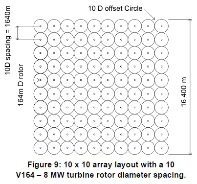
Using the array layout in Figure 9 in conjunction with Equation 7, the array density ρ was calculated to be 2.974 MW/Km².

 

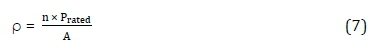
where n is the number of turbines; P_rated is the rated power of the V164 - 8 MW turbine; and A is the area of the wind farm.

To accurately determine the array density, the relevant efficiency losses experienced within a typical wind farm were considered. The efficiency losses assumed for this study are given in Table 3.

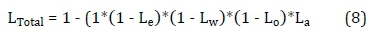
According to Musial et al. (2016), the total efficiency losses L_Total can be calculated using Equation 8. This equation results in a total wind farm loss of 19.41%. It must be noted that the wind farm losses are highly dependent on the wind farm layout and location. For simplicity, this study used an L_Total of 19.41% for all locations. This L_Total is validated by Musial et al. (2016) who published a standard L_Total range of 12-23%. Applying this L_Total to the array density of 2.974 MW/Km², calculated in Equation 7, yielded a more accurate array density of 2.397 MW/Km², which factors in all wind farm losses. This array density was used to determine the final AEP of the four developmental scenarios.

3.5 Annual energy production

The AEP estimate for each of the scenarios was made using Equation 9.

 

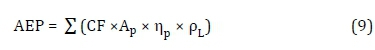
where AEP is the annual energy production; CF is the pixel capacity factor; A_p is the pixel area; r|_p is the number of pixels with a specific CF; and p_L is the array density after losses.

Table 4 shows a summary of the AEP estimates determined in this study, with the final AEP estimation for each scenario, as well as the power resource before and after wind farm losses are considered. The final AEP estimations for each of the scenarios is the AEP after subtracting the inaccessible resources that exists in protected regions.

 

4. Model validation and discussion

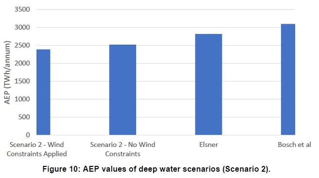
For the purpose of model and methodology validation, the AEP results generated in this study were compared against the AEP estimates from the OWE resource assessment studies in Table 1. It is expected that final AEP estimates will vary from study to study due to the methodology differences previously noted. Figure 10 compares the deep water AEP results generated from this study against those of Elsner (2019) and Bosch et al. (2018). This study estimated a similar South African deep water OWE resource to both of those. It was expected that this study would generate lower AEP values than both Elsner and Bosch et al. as it used a significantly lower final array density (see Table 1). The various other discrepancies in methodologies and input data highlighted in Table 1 led to variation in AEP results.

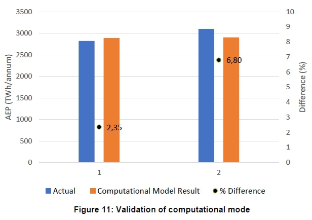
Eurek et al. (2017), in order to validate their computational model, compared the outputs generated from their computational model against the actual AEP results of similar studies. A similar validation approach was used here, where the inputs of this study were synced with those of Elsner. Els-ner's final array density and minimum wind speed quality (3 MW/km² and 7.5 m/s at 100 m ASL respectively) were modelled as new inputs into the current study's AEP computational model. The result from this iteration was a final AEP estimation of 2 889 TWh, which is a mere 2.4% higher than Els-ner's actual AEP estimation. This served as a fair validation of the methodologies and computational model used in the current study. The negligible difference of 2.4% can be ascribed to other differences between the two studies, such as wind data sources and scenario depth limits.

A similar validation procedure was performed using input parameters from Bosch et al. (2018). When using their input parameters in the current study's AEP computational model, the output AEP value determined was 6.8% lower than that calculated by Bosch et al. This too, served as a fair validation of this study's methodology and computational model. The results of the validation procedure are displayed in Figure 11.

 

5. Offshore wind farm site selection

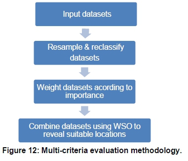
This paper adopted a GIS-based multi-criteria evaluation (MCE) technique to identify the most suitable offshore wind development sites within the South African EEZ. The MCE methodology shown in Figure 12 generates a spatially accurate suitability map, which pinpoints the most suitable offshore wind development regions. The suitability map essentially displays a unique suitability score for each pixel resolution. The pixel specific suitability scores were used for the fabrication of the suitable development region site maps shown in Figures 14, 15 and 16.

 

 

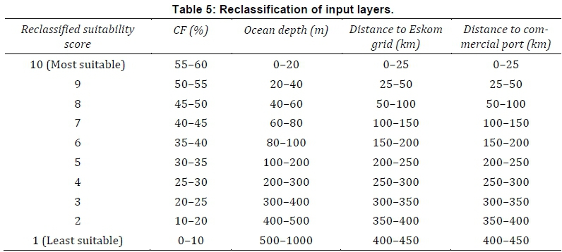
Input data layers used in the MCE were: capacity factor, ocean bathymetry, distance from existing Eskom transmission grid, and distance to commercial harbours. The input data layers were resampled using the nearest-neighbour technique in ArcGIS to match the pixel size of the highest resolution input data layer. The input data layers were resampled to the ERA5 wind speed pixel resolution of 461.5 m x 461.5 m (in the WGS_1984_UTM _Zone_35S coordinate system). Next, these input layers were reclassified to a common suitability scale of 1-10, with 1 being the least suitable and 10 being the most suitable. The reclassification of the input layers was performed according to Table 5.

The MCE methodology required the combination of spatial and non-spatial data (inputs) for the computation of a resultant decision (output). The procedure involves using geographical data, and the decision-maker's preferences (Malczewski, 2004). The reclassification shown in Table 5 represents the author's (decision-maker's) subjective data reclassification. The most suitable values of each of the data layers received a reclassified suitability score of 10/10; similarly the least suitable values of each input data layer received a reclassified suitability score of 1/10. The intermediate data values were reclassified on an approximate linear scale, with the exception of ocean depth which followed a rough logarithmic scale.

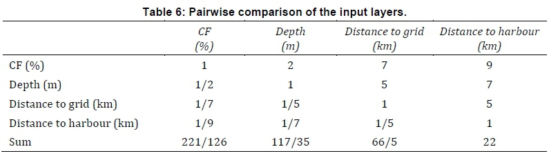
The reclassified input layers were then weighted according to importance. The layer weightings were determined using the analytical hierarchy process (AHP) methodology, as it offers a structured approach to rating criteria according to importance (Saaty, 1980). The AHP generates a weighting for each evaluation criterion according to the decision-maker's pairwise comparison of the criteria. Saaty (1980) offers a fundamental rating scale ranging from 1-9, with 1 representing equal importance and 9 representing superior importance. The pairwise comparison used in this study is shown in Table 6.

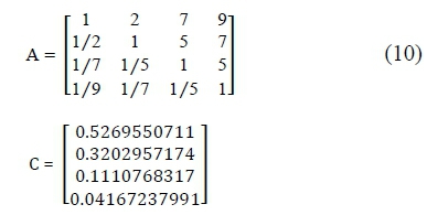
Maintaining the structure of Table 6, the initial comparison matrix was constructed. This comparison matrix labelled A is displayed in Equation 10. To determine the final layer weightings, each column was first normalised, by dividing each column by its respective summations.

Next, the normalised principle eigenvector was obtained by averaging across the rows of the normalised matrix (Saaty, 1980). This normalised principle eigenvector is also known as the priority vector. It is used in the final step of the MCE to determine the final suitability map.

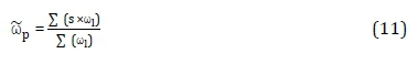
The final step of the MCE was accomplished using the weighted sum overlaying tool in ArcGIS. This tool stacks a series of input raster layers on top of one another to determine the most suitable raster pixels. Thus, each pixel in the input layers had a unique spatial coordinate, reclassified suitability value and relative importance weighting. The weighted sum overlay tool generated a final suitability factor map, technically known as a weighted-average map, by numerically combining both the reclassified suitability value of each pixel s and layer weighting ω₁, whilst maintaining each pixel's spatial accuracy. This gives the final weighted average value for each pixel, numerically illustrated in Equation 11.

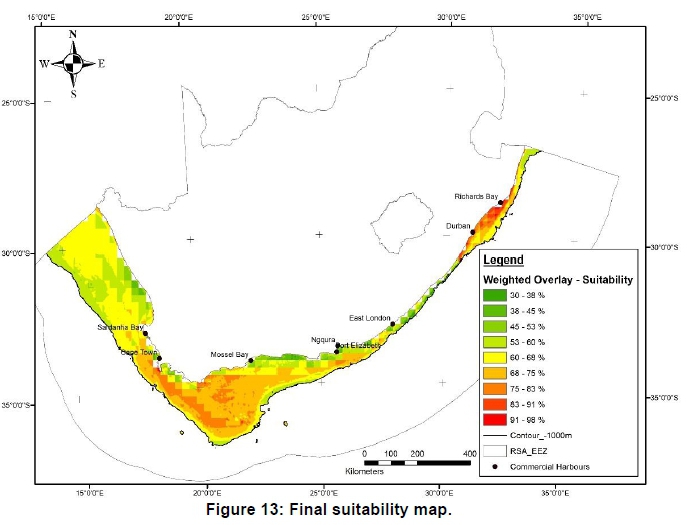
The final weighted average/suitability map is shown in Figure 13. This map shows the suitability of each pixel, in percentage, for the development of offshore wind. Due to the technical reasons already explained, pixels at depths of greater than 1 000 m are not included in this map. The areas of darker orange and red represent the most suitable locations for the development of offshore wind within South Africa's EEZ.

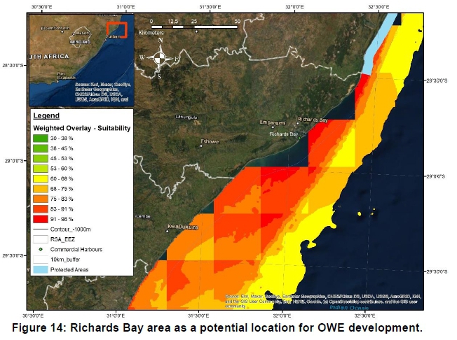
Figure 14 reveals the most suitable region for offshore wind development within the South African EEZ, the Richards Bay area. It illustrates suitability factors of up to 98% within close proximity to the coastline. Other data layers, such as protected regions and policy constraints, need to be considered in conjunction with the suitability map - for the selection of suitable offshore wind development sites. The map displays protected regions, and the 10 km buffer accounted for earlier, but it still displays significant potential for OWE development as there remain suitability pixel values of between 91% and 98% beyond the buffer. Highly suitable pixels between 91% and 98% exist in the waters between Richards Bay and KwaDukuza just beyond the 10 km buffer. Furthermore, these potential OWE developmental pixels are in a relatively shallow low depth range of 40-60 m. This will allow the deployment of cheaper fixed-bottom OWE foundations, thus increasing the attractiveness of this site.

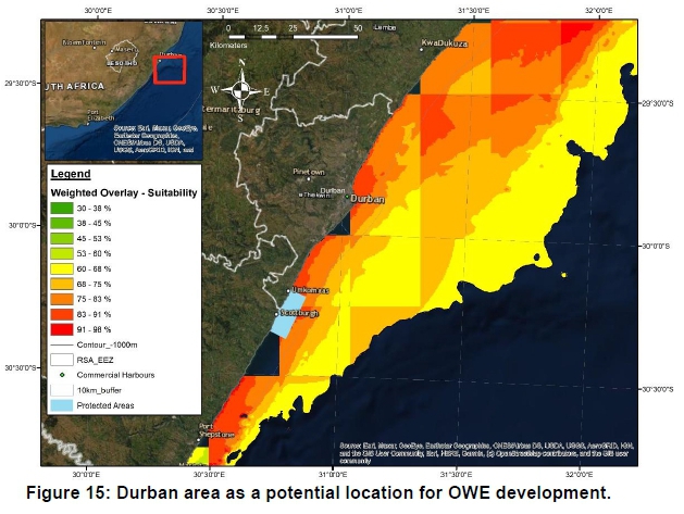
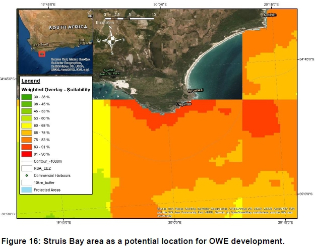
Figure 15 shows another of the regions with significant opportunity. Based on the high suitability percentages shown in Figure 15, the waters around Durban are arguably the second-best location for offshore wind development. The map reveals an abundance of pixels with suitability scores of 83-91% between Durban and KwaDukuza just beyond the 10 km buffer. Figure 16 shows the third suitable location for OWE development. East-southeast of Struis Bay lies a collection of pixels approximately 10 km x 10 km with a suitability factor of 83-91%.

 

6. Conclusions

This study is based on the importance of decoupling carbon emissions from electricity generation. South Africa has an ageing coal power fleet, which, over the next 30 years, will slowly be decommissioned.

This creates significant opportunity for this electricity generation gap to be filled with renewable energy technologies. The global offshore wind energy (OWE) industry is currently on the rise, with significant growth occurring in Europe and Asia.

The industry growth is maturing the technology and slowly reducing costs.

Due to the development of this industry, a number of global OWE resource assessments studies have been conducted. A number of these studies highlight the OWE resource potential available to South Africa (Bosch et al., 2018; Elsner, 2019; Eurek, Sullivan, Gleason, Hettinger, Heimiller & Lopez, 2017). This study conducted an OWE resource assessment of South Africa with the goal of validating, expanding on and potentially improving the existing OWE resource assessment literature.

This study has established that there is significant OWE resource available within South Africa's exclusive economic zone (EEZ). The OWE resources available to South Africa have been quantified under four unique developmental scenarios. Scenario 1 reveals the OWE resources available to South Africa within shallow waters. These resources can be harnessed using fixed-bottom OWT technology. Scenario 2 illustrates the OWE resources in deep waters; the majority of the resources available in Scenario 2 would need to be harnessed using floating OWT technology. Scenario 1^a and Scenario 2^a illustrate the OWE resources available once, and if, a restrictive policy is implemented. The annual energy production (AEP) estimates determined by this study are summarised below. They were calculated with the minimum wind quality limitations applied:

• Scenario 1: 44.52 TWh available at depths less than 50 m.

• Scenario 2: 2 387.08 TWh available at depths less than 1 000 m.

• Scenario 1^a: 15.42 TWh available at depths less than 50 m with the restrictive policy applied.

• Scenario 2^a: 2 321.54 TWh available at depths less than 50 m with the restrictive policy applied.

According to Eskom (2019), South Africa's annual electricity consumption is approximately 297.8 TWh. By converting the above AEP figures to a percentage of South Africa's annual electricity consumption, it is calculated that the estimated AEP for Scenario 1 could theoretically meet 14.9% of South Africa's electricity demand. Similarly, the estimated AEP available in Scenario 2 could theoretically satisfy South Africa's annual electricity demand eight times over. Based on the findings of this study, it is clear that OWE has significant potential to play a fundamental role in South Africa's future power security and decarbonisation strategies.

 

Author contributions

G. Rae was responsible for the literature review, methodology design, data collection, model configuration, data analysis, ArcGIS mapping, and manuscript write-up. G. Erfort was responsible for methodology validation, model verification, and manuscript quality control.

 

Acknowledgements

The authors thank Dr Chris Lennard and Mr Pierre Kloppers from The University of Cape Town's Climate System Analysis Group for their assistance with Climate Data Organiser. Additional gratitude is extended to Ms Caley Higgs from Stellenbosch University's Geoinformatics Department, for her willingness to assist with ArcGIS-related queries.

 

References

Andrews, J. and Jelley, N. 2007. Energy science: Principles, technologies, and impacts. Oxford: Oxford University Press.         [ Links ]

Ang, B.W. and Su, B. 2016. Carbon emission intensity in electricity production: A global analysis. Energy Policy 94:56-63.         [ Links ]

Bauer, L. amd Matysik, S. 2019. Vestas V164-8.0 - 8,00 MW- Wind turbine. Available online at https://en.wind-turbine-models.com/turbines/318-vestas-v164-8.0 [2019, October 03].         [ Links ]

Bosch, J., Staffell, I. and Hawkes, A.D. 2018. Temporally explicit and spatially resolved global offshore wind energy potentials. Energy 163:766-781.         [ Links ]

Busby, R. (2012). Wind power - the industry grows up. Available online at https://app.knovel.com/web/view/khtml/show.v/rcid:kpWPTIGU01/cid:kt00C4HSM3/viewerType :khtml/?page=1andview=collapsedandzoom=1andq=rayleighwindspeeddistribution [2019, May 02].         [ Links ]

Copernicus Climate Change Service (C3S). 2017. ERA5: Fifth generation of ECMWF atmospheric reanalyses of the global climate. Copernicus Climate Change Service Climate Data Store. Available online at https://cds.climate.co-pernicus.eu/cdsapp#!/home [2019, June 19].         [ Links ]

DOE [Department of Energy]. 2019. IPP Projects. Available online at https://www.ipp-projects.co.za/ [2019, April 19].         [ Links ]

Dupont, E., Koppelaar, R. and Jeanmart, H. 2018. Global available wind energy with physical and energy return on investment constraints. Applied Energy 209 (September 2017): 322-338.         [ Links ]

Dvorak, M.J., Archer, C.L. and Jacobson, M.Z. 2010. California offshore wind energy potential. Renewable Energy 35(6): 1244-1254.         [ Links ]

Elsner, P. 2019. Continental-scale assessment of the African offshore wind energy potential: Spatial analysis of an under-appreciated renewable energy resource. Renewable and Sustainable Energy Reviews 104(January): 394407.         [ Links ]

Eurek, K., Sullivan, P., Gleason, M., Hettinger, D., Heimiller, D. and Lopez, A. 2017. An improved global wind resource estimate for integrated assessment models. Energy Economics 64: 552-567.         [ Links ]

Fakir, S. 2015. COP 21 and South Africa's position. Engineering News. Available online at www.engineering-news.co.za/article/cop-21-and-south-africas-position-2015-10-09 [2019, June 8].         [ Links ]

Flanders Marine Institute. 2014. Union of the ESRI Country shapefile and the Exclusive Economic Zones (version 2). Available online at http://www.marineregions.org/. [2019, September 24].         [ Links ]

Hartley, F., Ireland, G., Merven, B., Burton, J., Ahjum, F., McCall, B., Caetano, T., Wright, J., et al. 2017. The developing energy landscape in South Africa: Technical Report. (October). Available online at http://www.erc.uct.ac.za/sites/default/files/image_tool/images/119/Researchdocs/ERC [2019, March 12].         [ Links ]

Hennermann, K. 2019. What is ERA5 - Copernicus Knowledge Base - ECMWF. Available online at https://confluence.ecmwf.int/display/CKB/WhatisERA5 [2019, September 24]        [ Links ]

Hong, L. and Möller, B. 2011. Offshore wind energy potential in China: Under technical, spatial and economic constraints. Energy 36(7): 4482-4491.         [ Links ]

Malczewski, J. 2004. GIS-based land-use suitability analysis: A critical overview. Progress in Planning 62(1): 3-65. doi: 10.1016/j.progress.2003.09.002.         [ Links ]

McGlade, C. and Ekins, P. 2015. The geographical distribution of fossil fuels unused when limiting global warming to 2 °C. Nature 517, 187-190.         [ Links ]

Meinshausen, M., Meinshausen, N., Hare, W., Raper, S., Frieler, K., Knutti, R., Frame, D. and Allen, M. 2009. Greenhouse- gas emission targets for limiting global warming to 2 °C. Nature 458:1158.         [ Links ]

Musial, W., Heimiller, D., Beiter, P., Scott, G. and Draxl, C. 2016. Offshore wind energy resource assessment for the United States. (September): 88.         [ Links ]

Rae, G. 2019. Offshore wind energy resource assessment of the South African exclusive economic zone. Unpublished Masters thesis. Stellenbosch: Stellenbosch University.         [ Links ]

Saaty, T.L. 1980. The analytic hierarchy process: Planning, priority setting, resource allocation. European Journal of Operational Research 9(1): 97-98.         [ Links ]

UNEP-WCMC. 2019. Protected area profile for South Africa from the world database of protected areas, October 2019. Available online at www.protectedplanet.net. [2019, May 17].         [ Links ]

UNFCCC. 2015. Adoption of the Paris Agreement. Experimental Mechanics 8(11): 513-519.         [ Links ]

Weatherall, P., Marks, K.., Jakobsson, M., Schmitt, T., Tani, S., Arndt, J.., Rovere, M., Chayes, D., et al. 2015. A new digital bathymetric model of the world's oceans. Earth and Space Science, 2. doi: 10.1002/2015EA000107        [ Links ]

Yamaguchi, A. and Ishihara T. 2014. Assessment of offshore wind energy potential using mesoscale model and geo graphic information system. Renewable Energy 69: 506-15. https://doi.org/10.1016/j.renene.2014.02.024.         [ Links ]

 

 

* Corresponding author: Tel: +27 (0)72 913 1117; email: gordonrae95@gmail.com