ARTICLES

 

Intelligent techniques, harmonically coupled and SARIMA models in forecasting solar radiation data: A hybridisation approach

 

 

K. S. Sivhugwana; E. Ranganai^*

Department of Statistics, University of South Africa, Roodepoort, South Africa. 1. ORCiD: https://orcid.org/0000-0002-6536-4046 2. ORCiD: https://orcid.org/0000-0002-2428-5405

 

 

---

ABSTRACT

The unsteady and intermittent feature (mainly due to atmospheric mechanisms and diurnal cycles) of solar energy resource is often a stumbling block, due to its unpredictable nature, to receiving high-intensity levels of solar radiation at ground level. Hence, there has been a growing demand for accurate solar irradiance forecasts that properly explain the mixture of deterministic and stochastic characteristic (which may be linear or nonlinear) in which solar radiation presents itself on the earth's surface. The seasonal autoregressive integrated moving average (SARIMA) models are popular for accurately modelling linearity, whilst the neural networks effectively capture the aspect of nonlinearity embedded in solar radiation data at ground level. This comparative study couples sinusoidal predictors at specified harmonic frequencies with SARIMA models, neural network autoregression (NNAR) models and the hybrid (SARIMA-NNAR) models to form the respective harmonically coupled models, namely, HCSARIMA models, HCNNAR models and HCSARIMA-NNAR models, with the sinusoidal predictor function, SARIMA, and NNAR parts capturing the deterministic, linear and nonlinear components, respectively. These models are used to forecast 10-minutely and 60-minutely averaged global horizontal irradiance data series obtained from the RVD Richtersveld solar radiometric station in the Northern Cape, South Africa. The forecasting accuracy of the three above-mentioned models is undertaken based on the relative mean square error, mean absolute error and mean absolute percentage error. The HCNNAR model and HCSARIMA-NNAR model gave more accurate forecasting results for 60-minutely and 10-minutely data, respectively.
HIGHLIGHTS:
• HCSARIMA models were outperformed by both HCNNAR models and HCSARIMA-NNAR models in the forecasting arena.
• HCNNAR models were most appropriate for forecasting larger time scales (i.e. 60-minutely).
• HCSARIMA-NNAR models were most appropriate for forecasting smaller time scales (i.e. 10-minutely).
• Models fitted on the January data series performed better than those fitted on the June data series.

Keywords: forecasting, harmonic frequencies, SARIMA models, NNAR models, SARIMA-NNAR models

---

 

 

1. Introduction

Alongside a rapid and continuous decline in the cost of clean energy harvesting systems (i.e. solar panels and wind turbines), the cost of generating solar power is also anticipated to decline by more than 50% in the next seven years (International Renewable Energy Agency, 2016). Among renewable energy resources (e.g. water, solar and wind), solar power is expected to have the highest levels of unexplored potential for a wide spectrum of applications, due to the interminable nature and abundant availability of sunlight (Suleiman and Adejumo, 2017; Reddy et al, 2017). Hence, the integration of large volumes of solar energy into electricity grids is constantly increasing (Diagne et al, 2013). However, the continuous varying nature of solar energy resource (i.e. solar radiation), can pose a great challenge to this integration, thereby compromising the reliability and stability of the electricity grid (Chu et al, 2015). The varying and intermittent feature (mainly due to atmospheric mechanisms and diurnal cycles) of solar radiation is often a stumbling block (due to its unpredictable nature) to receiving high-intensity levels of solar radiation on the ground level, thereby lowering the levels of solar power being harvested and penetrating the existing electricity network (Lorenz et al, 2004; Chu et al., 2015; Voyant et al, 2017). This further complicates the process of forecasting solar radiation and destabilises the efficiency and effectiveness of the solar resource to penetrate the electricity power grid (Chu et al, 2015). Moreover, it leads to high voltage variations, which compromise the quality of power generated and distributed, as well as increase the cost of generating power reserves (Voyant et al, 2017).

For maximum application in sizing and designing solar energy harvesting instruments (e.g. photovoltaic (PV) systems) or predicting the prospective solar power farms or high integration of solar power into the electrical network and effective operation of the electricity grid, solar irradiance must be well-defined and be accompanied by accurate forecasts at various time horizons (ranging from minutes to years) (Martin et al, 2015; Pavlovski and Kostylev, 2011). At present, different solar forecasting methodologies (e.g. time series, machine learning, artificial intelligence, etc) have been developed and applied at different forecasting time-scales to meet the increasing demand for more effective predictive ability for solar radiation (Chu et al, 2015) (also see Martin et al, 2015; Chaturvedi and Isha, 2016; Reddy et al, 2017; Voyant et al, 2017; Voyant et al, 2011).

This study is, however, concerned with short-term forecasting.

Among the time series-based forecasting methods, the Box-Jenkins non-seasonal/seasonal autoregressive integrated moving average (S/ARIMA) model has been widely applied in forecasting solar irradiance, because of its ability to handle linearity, seasonality and the stochastic component embedded in solar radiation data (see Mukaram and Yusof, 2017; Ranganai and Nzuza, 2015). On the other hand, artificial neural networks (ANNs) from the family of artificial intelligence (Chaturvedi & Isha, 2016; Voyant et al, 2011) are known to be very flexible and nonlinear, with the capacity to capture the nonlinear characteristics inherent in solar radiation data that cannot be properly explained by traditional models (e.g. SARIMAs) (Mukaram and Yusof, 2017; Zhang, 2003; Bozkurt et al, 2017). However, no clear-cut conclusion has been reached in determining which is the better model - ANN or S/ARIMA (see Mukaram and Yusof, 2017; Zhang, 2003), due to the unpredictable mixture of deterministic and stochastic (which may be linear and nonlinear) components that often characterises time series data in real-world situations. Hence, Zhang (2003) proposed blending ARIMAs and ANNs to form ARIMA-ANN hybrid models to capture linear and nonlinear characteristics often infused in the time series data. Ranganai and Nzuza (2015) proposed an even better modelling approach, of capturing both the deterministic and stochastic components through coupling sinusoidal predictors at determined harmonic (Fourier) frequencies with the SARIMA model to form the HCSARIMA model. In this procedure, they first impose sinusoidal predictors on the irradiance data to capture the major seasonal component. Thereafter, the SARIMA model was fitted on the residuals to handle the stochastic component. The HCSARIMA model was found to be effective at reducing the forecasting error, particularly when dealing with a longer horizon (two days ahead). The study results showed that the HCSARIMA model is superior to the SARIMA model in forecasting global horizontal irradiance (GHI) data recorded on the earth's surface. Motivated by these results, the current study aims to determine whether the HCSARIMA model has a competitive edge over other potential harmonically coupled models, specifically the harmonically coupled NNAR (HCNNAR) model and SARIMA-NNAR (HCSARIMA-NNAR) model, in terms of improving the forecasting error. Thus, this study intends to employ the above-mentioned harmonically coupled models to effectively capture deterministic and stochastic com-ponents embedded in the solar irradiance data, with the sinusoidal predictor function, SARIMA and NNAR parts capturing the deterministic, linear and nonlinear components, respectively. To the knowledge of the authors, there is very limited, if any, work done on modelling and forecasting South African GHI data using HCNNAR and HCSARIMA-NNAR models. Researchers have used different models, such as quantile regression averaging (QRA), non-linear multivariate models, multilayer perceptron neural network (MLPNN), radial basis function neural network (RBFNN) and physical ap-proaches (see Mpfumali, et ah, 2019; Govinda-samy and Chetty, 2019; Zhandire, 2017; Kibirige, 2018).

The GHI data series modelled in this paper covers the two months of January (summer) and June (winter) 2017, collected from RVD Richtersveld radiometric station, located at 28.56° South, 16.76° East about 30 km East with 140 m elevation, at Alexandra Bay, Northern Cape province, South Africa. Each of the data series is averaged at a 10-minutely and 60-minutely time scale. The RVD Richtersveld radiometric station is equipped with a Kipp & Zonen radiometer that is attached to the SOLYSIS tracker (Brooks et al, 2015). The SOLYSIS tracker consists of CHP1 pyrhelio-meters to measure direct normal irradiance (DNI), and CMP11 pyranometers to measure both GHI and diffuse solar irradiance (DHI).

The rest of the paper is organised as follows. In Section 2, a brief overview of SARIMA models is presented, while a summary of NNAR models is given in Section 3. Section 4 presents the periodogram analysis and shows how it can be coupled with other models. In Section 5, a harmonically coupled modelling is presented, whilst in-sample diagnostics, as well as out-of-sample diagnostics, are discussed in section 6. Section 7 focuses on the description and analysis of various data series and empirical results. Discussion of the results and conclusions are given in Section 8 and Section 9, respectively.

 

2. SARIMA models

SARIMA models belong to one of the most-utilised forecasting techniques for analysing time series data, probably because they offer great flexibility and accurate forecasts (Zhang, 2003). This technique uses a linear combination of historical observations to accurately predict future time series observations, and also performs analysis on the univariate stochastic time series (i.e. innovations). As such, stationarity (i.e. mean, variance and covariance must remain constant over time) is necessary for these models to produce accurate forecasts (Khalek and Ali, 2015). SARIMA models combine three processes: an autoregressive (AR) process, integrated or differencing (I) to ensure data stationarity and remove seasonality, and a moving average (MA) process. The general form of SARIMA model is denoted by SARIMA (p,d,q) X (P,D,Q)_Smodel, which is given by Equation 1 (see Box et al, 1994; Hyndman and Athanasopoulos, 2013; Box and Jenkins, 1976).

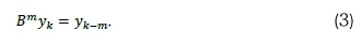
where µ_y is a constant; Φ_p(B) = l-BΦ₁-ß²Φ₂-...-ß^pΦ_p (AR polynomial); 0_q(B) = 1-B0₁ -B²0₂-...-B^q0_q(MA polynomial) ; p (order of non-seasonal AR process); d (number of non-seasonal differencing); q (order of non-seasonal MA); Φ_P(B^s) = 1-B^sΦ₁-B^2sΦ₂-...-B^2pΦ_p(seasonal AR polynomial); 0_Q(B^s) = 1 - B^s0₁ -B^2s0₂-...-B^sqO_q(seasonal MA polynomial); P (order of seasonal AR); D (number of seasonal differencing); Q (order of seasonal MA); s (seasonality); y_k(time series or stochastic process at time lag k); e_k ~ N (0, σ²) (i.e. Independent and identically distributed (IID) white noise process with mean of zero and constant variance); V_S^D (seasonal difference); V^d (non-seasonal difference); and B (back-shift operator). The roots of the polynomials 0(B) = 0 and Φ(ß) = 0 must lie outside the unit circle (Wei, 1990). The back-shift operator (B) is defined as a linear operator that shifts the time index one period back such that:

and

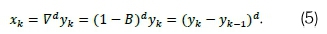
The order of differencing (d) ensures data stationarity is defined as:

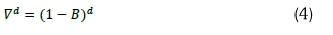
such that a stationary time series {x_k} that has been differenced d times is given by:

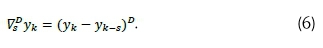
Seasonally differenced time series {y_k} is given by:

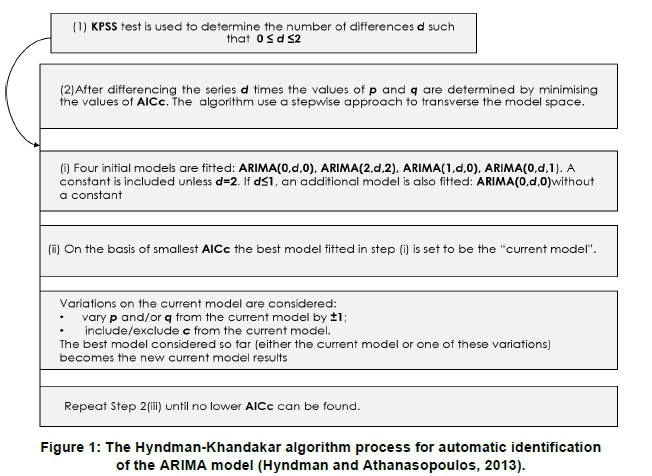
The Hyndman-Khandakar algorithm is applied using the auto.arima function in R to search for an optional ARIMA model. To find the most appropriate ARIMA model, the algorithm applies the maximum likelihood estimation (MLE), the Kwiatkowski-Phillips-Schmidt-Shin (KPSS) test for the unit root testing, and the corrected Akaike Information Criterion (AIC) (i.e. AIC with correction for small sample sizes) (Hyndman and Athanasopoulos, 2013). The corrected AIC (or AICc) addresses the potential of model over-fitting. For a large sample size, AICc will ultimately converge to AIC. The Hyndman-Khandakar algorithm for automatic identification of the ARIMA model is diagrammatically illustrated in Figure 1.

When handling seasonal data, the auto.arima function uses ndiffs function to calculate the appropriate number of first order differences (d). Similarly, D the number of seasonal differencing, is determined using nsdiffs function. The rest of the seasonal parameters P and Q are identified by minimising AICc.

 

3. NNAR analysis

Artificial neural networks (ANNs) are nonlinear and nonparametric models that are often applied in machine learning (Zhang, 2003; Sena and Nagwani, 2016). These methods provide the best results when predicting functions based on a larger sample of the training set (Sena and Nagwani, 2016). According to Zhang (2003), ANNs have several advantages over linear models (e.g. SARIMA models) in time series forecasting, because they are data-driven and have self-adaptive techniques. As such they rarely require prior theoretical model assumptions about the data under investigation. ANNs are also able to learn, memorise and recognise patterns without any temporal relations in the data, and model a phenomenon to any desired accuracy level (Pretorius and Sibanda, 2012; Fonseca et al, 2011).

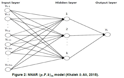
ANNs are machine-learning techniques that are biologically inspired by the human neural processing system (Sena and Nagwani, 2016; Pretorius and Sibanda, 2012). These techniques consist of algorithms (e.g. back-propagation algorithm) that mimic the structure of the human brain to process data using a network of highly connected (through weights) nodes or neurons (Pretorius and Sibanda, 2012; Baridam and Irozuru, 2012). The weights lie within the values of -1 and +1. Inhibitory (negative) weight decreases the total input value into a neuron, while excitatory (positive) weight increases the total input into a neuron. The network is interlinked in the distinguishable layer of the topology of neurons. The network constitutes three main layers of neurons, namely, the input layer (which is the first layer in the network), the hidden layer (middle layer of the network), and the output layer (the final layer of the network) (Pretorius and Sibanda, 2012; Fonseca et al, 2011; Baridam and Irozuru, 2012).

Training of the network using a larger volume of training data sets plays a significant role in implementing successful ANNs. With the aid of the back-propagation algorithm, ANNs learn to adjust weights associated with each connection within the network during the training stage (Hyndman and Athanasopoulos, 2013). The rationale behind the training is to find a set of weights such that the difference between the calculated output by the ANN model and the known targeted value is as small as possible (Hyndman and Athanasopoulos, 2013; Pretorius and Sibanda, 2012).

The feed-forward neural networks present the most basic and simple form of ANN architectures, where the signal is only able to flow in a forward direction, from the input neurons, through the hidden neurons to the output neurons (Sena and Nagwani, 2016; Pretorius and Sibanda, 2012; Fonseca et al, 2011; Baridam and Irozuru, 2012). There are two types of feed-forward neural networks, namely single-layer perceptron network and MLPNN (Mukaram and Yusof, 2017; Pretorius and Sibanda, 2012). The single-layer feed-forward network (which is the simplest network that contains no hidden layers and is equivalent to linear regressions (Hyndman and Athanasopoulos, 2013) consists of inputs, single-layer, output, and a bias term. MLPNN feed-forward networks consist of at least three layers consisting of a single input layer and an output layer with at least one hidden layer depending on the problem under investigation (Mukaram and Yusof, 2017; Hyndman and Athanasopoulos, 2013; Pretorius and Sibanda, 2012).

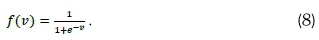
NNAR model is a type of MLPNN feed-forward network with one hidden layer and logistic sigmoid as an activation function to minimise the overall impact of extreme values on the predicted final output (Hyndman and Athanasopoulos, 2013; Khalek & Ali, 2015). Contrary to linear autoregression models such as SARIMA models, the NNAR model utilises historically lagged data series as inputs into the neural network for forecasting and has no restrictions on the model parameters to ensure stationarity (Hyndman and Athanasopoulos, 2013). This feed-forward technique involves a linear combination function (of the inputs) and nonlinear sigmoid activation function (usually a logistic function) (Khalek & Ali, 2015; Hyndman and Athanasopoulos, 2013).

Inputs into the network are combined linearly and the output is passed through the sigmoid function (Khalek & Ali, 2015; Fonseca et al, 2011). Thus, the total input into the j^thneuron is the weighted sum of all the outputs from all other earlier neurons connected to it and is calculated as follows:

where w_ij denotes the weight connecting neuron i to neuron j, y_i. is the output of neuron i, b_jis the threshold coefficient for neuron j, m is the number of neurons in the hidden layers, and f (which modifies the input V_jin the hidden layer) is a nonlinear logistic sigmoid function such that (Hyndman and Athanasopoulos, 2013):

If the input value into a neuron is above the threshold b_j(i.e. the standardised input to a neuron in the absence of any other inputs) the neuron will fire, otherwise, it will not fire (i.e. reject the value).

When applied on non-seasonal time series data to forecast output y_t, the NNAR model is denoted by NNAR (p, k), with p being the number of lagged inputs and k the number of neurons in the hidden layers (Hyndman and Athanas-opoulos, 2013). For the application on seasonal time series data, the NNAR model is denoted by the notation NNAR (p,P,k)_m, where P is the seasonal AR order, {y_t-1,y_t-2,..., y_t-_m, y_t-_2m, y_t-pm}are the lagged values, k is the number of neurons in the hidden layer, and seasonality at multiples of m (see Figure 2). For example, NNAR (4,1,14)₁₂ has {y_t-1,.y_t-2, y_t-3, y_t-4, y_t-14} inputs with 14 neurons in the hidden layers and seasonality at multiples of 12. Without the existence of the hidden layer, the NNAR model is given by NNAR (p,P, 0)_m, which is analogous to ARIMA (p,0,0)(P,0,0)_m (Hyndman and Athanasopoulos, 2013). Since the data at RVD Richtersveld radiometric solar station are expected to have some aspects of seasonality, the function nnetar in R program will be used to automatically fit the best NNAR (p,P,k)_mmodel. This function selects the autoregressive seasonal parameter, P=l by default, with the non-seasonal autoregressive parameter or number of lagged outputs p being extracted from the fitted optimal linear SARIMA model. If k is not selected, it can be calculated by Equation 9:

 

 

 

When it comes to forecasting using the NNAR model, the network is applied iteratively. For a step-ahead forecast, the NNAR model uses available historical observations as inputs into the network. For two-steps-ahead forecasts, the NNAR model combines both the available previous observations and computed one-step head forecasts as inputs into the network (Hyndman and Athanasopoulos, 2013). The process continues until all required forecasts are computed.

 

4. Periodogram analysis

When dealing with cyclic data, periodicity plays a significant role in unpacking the inherent characteristics of the data. Periodogram analysis is utilised in solar irradiance forecasting to explain the aspect of diurnal cycles (Ranganai and Nzuza, 2015). The periodogram, which is a well-known and widely applied fundamental nonparametric tool for detecting periodicities, is a spectrum estimation instrument that utilizes the fast Fourier transform (FFT). Statistically significant periodogram ordinates identify dominant frequencies or periods, which helps to determine dominant cyclic behaviour in the time

series data (Yarmohammadi, 2011). This frequency domain technique is also used in statistics to build statistical inference for spectral density function because its statistical characteristics are known (Yarmohammadi, 2011). For a real-valued time series {y_k} of length n, the periodogram I_n(v_p) is given by:

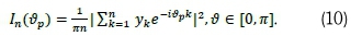
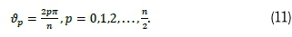
The periodogram can be calculated for a discrete data set at harmonic frequencies:

Suppose that a real-valued time series {y_k} contains a periodic sinusoidal component with a known wavelength given by (see Ranganai and Nzuza, 2015):

where v (measured in radians is such that n radians=180°) is the frequency of the sinusoidal variation, A is the amplitude of the variation, Φ is the phase and e_kis Gaussian white noise process with zero mean and unit variance. Frequency, denoted by f = is defined as the number of cycles per unit time and is used to explain the results of the data process. The period or wavelength is calculated as a function of the frequency and is given by - or The mathematical expression presented in Equation 12 can equivalently be written as Equation 13 (see Ranganai and Nzuza, 2015):

where a = Asin(Φ), ß = Acos(Φ) and µ_k = 0. In practice, the sinusoidal predictor function of the times series {y_k} may contain cyclical variations at different time scales (e.g. daily, weekly, etc.). To accommodate such instances Equation 13 is generalized as follows (see Ranganai and Nzuza, 2015; Yarmohammadi, 2011):

where a_j- = A_jcos(Φj) and b_j = -A_Jsin(Φj).

The existence of multiple periodic components or sharp peaks in the periodogram does not necessarily imply that each of these peaks corresponds to an actual sinusoidal component of the series. If a time series has a significant sinusoidal component with harmonic frequency _vk, the periodogram will have the highest peak at v_k. We can use Equation 14 to test the hypothesis whether the parameters a and b are zero at v_k, i.e. H0: a_k = b_k = 0 vs H_a: a_k0 or b_k 0 using Fisher's exact test. This assists in determining whether the value of the periodogram's peak is greater than that which is likely to rise in a model without true or actual sinusoidal components (i.e. white noise series) (Yar-mohammadi, 2011; Liew et al., 2009). Thus, the test determines whether a peak in the periodogram is significant or not. The standard procedure for applying periodogram analysis requires that one plots periodogram ordinates at v_p= -,p = 0,1,2, ,- harmonic frequencies first, and then appfies Fisher's exact test to detect the magnitude of the largest peak using the g- test statistic presented in Equation 15 (Yarmohammadi, 2011):

For any given a level of significance we can use Equation 15 to find the critical value g_a, such that P{g > g_a) = a. If g > g_a, the null hypothesis is rejected and the conclusion is reached that the signal {y_k} has a specified sinusoidal or periodic component (Yarmohammadi, 2011; Wei, 1990). Alternatively, if the p-value given by P{g > g_a) is less than a, we reject the null hypothesis and conclude that the time series is not white noise (see Ahdesmaki et al, 2007; Liew et al, 2009). Thus, the time series exhibits some periodic expression pattern (i.e. the maximum peak in the periodogram is significant). In this study, we use the fisher.g.test function in GeneCycle package in the R program to determine the significance of any periodogram ordinate.

 

5. Harmonically coupled modelling

It is assumed that the GHI data series of interest originates from a mixture of deterministic and stochastic process given by Equation 16:

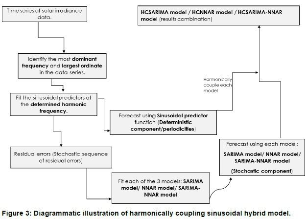
where y_kdenotes the predicted GHI data series, D_kis the deterministic component and S_kis the stochastic component. Harmonically coupled modelling consists of two main steps (Ranganai and Nzuza, 2015). The first step is where the data is modelled by the sinusoidal predictor function at the determined harmonic frequencies to capture the deterministic component. Thereafter, the sequence of residuals data (which could not be properly explained or captured by the sinusoidal predictors) are used as input into the SARIMA, NNAR and SARIMA-NNAR models to capture the stochastic component of the data. The final predicted value by the harmonically coupled model is the summation of the predicted value by the sinusoidal predictor function and the predicted value by either the SARIMA model /NNAR model/ SARIMA-NNAR model (see Figure 3).

For instance, we can derive HCNNAR models in the following two steps. Assume that GHI data series {y_k} is a mixture of deterministic component (D_k) and stochastic component (S_k) such that:

and

Step 1: Supposing e_kdenotes the residual at time lag k, then

where D_kis the forecasted value at time k using sinusoidal predictor model.

Step 2: Vector r=(e_k-1,e_k-2,...,e_{k_m}) of the residual errors obtained in step 1 are used as input data to the NNAR model with m nodes. After applying the NNAR model to the residual vector we obtain the following result (see Zhang, 2003):

where ƒ denotes the logistic sigmoid function and n_kis stochastic error. Thus, the HCNNAR model is a sum of the forecasted result by the sinusoidal predictor model and the NNAR model:

The HCSARIMA model is obtained in a similar fashion, by first injecting the residual error terms from the fitted sinusoidal predictor model into the SARIMA model (to capture the stochastic component). Thereafter, we combine the forecasting results by the sinusoidal predictor and SARIMA models to form the HCSARIMA model.

For the HCSARIMA-NNAR model, we first fit the sinusoidal predictor function on the GHI data series to capture the deterministic component. Thereafter; we inject the residual error terms from the fitted sinusoidal predictor function into SARIMA-NNAR model. In this way, the SARIMA model captures the linear part, while the NNAR model captures the nonlinear part (using the residual error terms generated from fitting SARIMA model as input into the neural network) of the stochastic component. Thereafter, we combine the forecasting results by the sinusoidal predictor model and SARIMA-NNAR model to form the HCSARIMA-NNAR model.

 

6. Model diagnostics

Model diagnostics employed comprise in-sample and out-of-sample diagnostics.

6.1 In-sample diagnostics

Model selection is based on the lowest values of the Bayesian information criterion (BIC), Akaike information criterion (AIC) and its corrected version AIC_C. AIC, AIC_C and BIC are respectively calculated by Equations 22-24 (Akaike, 1983; Hyndman and Athanasopoulos, 2013; Schwarz, 1978):

where n is the sample size; SSE is the sum of squares of the error terms; In is the natural logarithm; and k is the number of estimable parameter.

6.2 Out-of-sample diagnostics

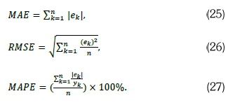
Prediction performance of all fitted models is assessed and compared using the well-known standard error metrics: mean absolute error (MAE) (in Watts per square metre (Wm^-2)), root mean square error (RMSE) (in Wm^-2), and mean absolute percentage error (MAPE) (in %). Smaller values of these performance metrics imply high accuracy forecasting ability of the model while high values are associated with poor forecasting ability. The error terms are denoted by e_k = [y_k - y_k), where k = 1,.., n; y_kand yk are the actual and predicted solar irradiance values at time k respectively (Zhang et al., 2013). Then, the forecasting accuracy measures are given by Equations 25-27:

 

7. Empirical results and discussion

7.1 Data source and exploratory data analysis

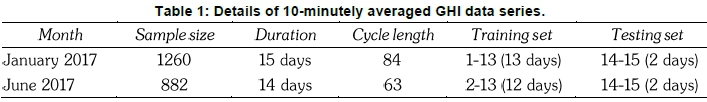
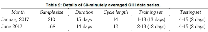
The GHI data series used in this study can be downloaded from the Southern African Universities Radiometric Network (SAURAN) website (http://www.sauran.net) (Brooks et al, 2015). All data records from SAURAN's RVD Richtersveld radiometric station are recorded by a sensor at sub-6 seconds intervals data readings and collected based on South African Standard Time (SAST) (Brooks et al, 2015). The 10-minutely averaged data used in this study were aggregated using the original one-minutely averaged data (see Table 1). The 60-minutely averaged data were readily available from the SAURAN website, but the same exercise of averaging was repeated to ascertain data quality (see Table 2).

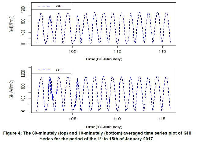
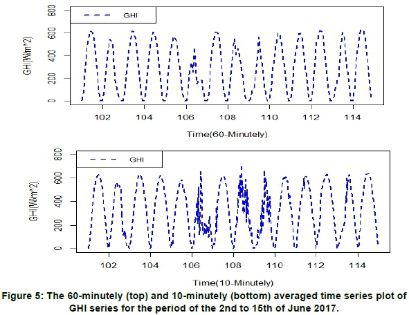
January 60-minutely averaged entries span from 06:00 am to 08:00 pm while 10-minutely averaged observations spans from 06:00 am to 08:10 pm. June 60-minutely averaged data spans from 07:00 am to 6:00 pm while 10-minutely averaged observations span from 07:30 am to 18:10 pm. Since summer months have hotter days and winter months have colder ones, larger values of irradiance are recorded for January, whereas lower values are recorded for June (see Figures 4 and 5). The time spans for both data series were deliberately chosen to accommodate as many daylight hours as possible while avoiding a high percentage of night and early morning zero values.

To evaluate the performance of the models, data were split into a training set (for model selection) and a testing set (to evaluate forecasting performance). The training set for the summer season covers the in-sample period of the 01st to 13th January 2017 and that of winter season covers the period of the 02nd to 13th June 2017. The testing set, on the other hand, constitutes two days out-of-sample period from the 14th to 15th for each of the two sampled months (see Table 1 and 2). The lower and upper limits time intervals for each day were kept the same to ensure stability in data modelling and forecasting throughout the analysis.

With affirmation from periodogram analysis, the seasonality on the 10-minutely data series was identified to be 84 and 63 data of 10 minutes per day for summer and winter periods respectively. In 60-minutely data, seasonal cycles were found to have a length of 12 hours and 14 hours per day for January and June, respectively. It was further observed that summer seasonal cycles are longer than winter ones, which is attributable to summer having longer days than winter.

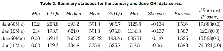
Table 3 shows the summary statistics for the January and June 2017 GHI data series. The minimum GHI value for January 10-minutely and 60-minutely time scales are 10.2 Wm^-2 and 0.3 Wm^-2, respectively. On the other hand, the June data series has a minimum GHI value of 0.0 Wm^-2 for each of the time scales of interest. January 10-minutely (1136.3 Wm^-2) and 60-minutely (1125.8 Wm^-2) time scales recorded the highest GHI values as compared to June 10-minutely (717.5 Wm^-2) and 60-minutely (635.51 Wm-2) time scales. The kurtosis for both January and June GHI data series is positive and it lies within the interval 1.5-1.6. This implies that both the January and June data series do not perfectly fit the normal distribution. Hence, the distributions of the four data series have heavier tails than the normal distribution. Except for the June 60-minutely time scale (which is positively skewed), the rest of the time scales have negatively skewed distributions. The means and the medians for all the time scales under investigation are unequal with p-values equals 0.0, which affirms that their distributions are not normally distributed.

7.2 Periodogram analysis

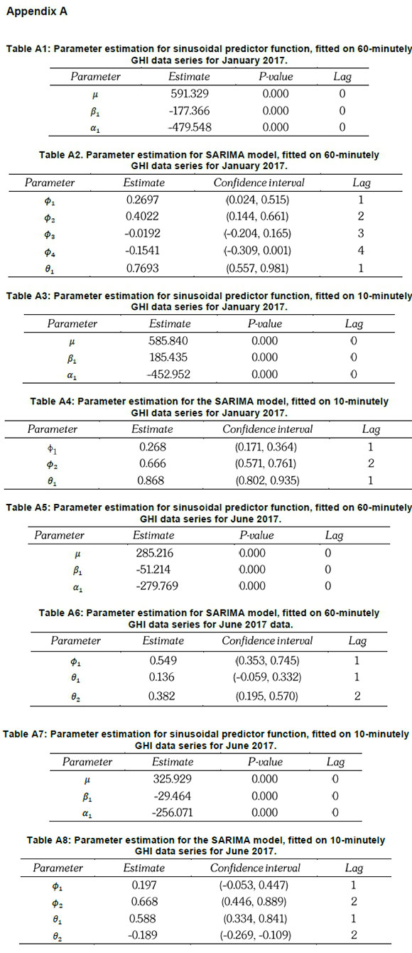
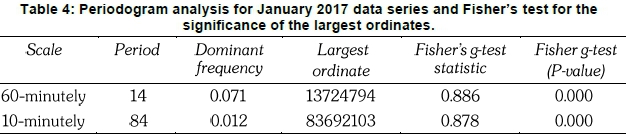
Figure 6 shows the diagrammatic representation of the largest ordinate at periods 14 and 84 for 60-minutely and 10-minutely averaged January data series, respectively. This corresponds to the harmonic frequency of 2r/14 for a 60-minutely time scale and 2r/84 for a 10-minutely time scale. Fisher's g-test statistic for the 60-minutely is equal to 0.886 while that of the 10-minutely data series is equal to 0.878. Both these statistics are significant (since p-value=0.00) at 1% level of significance, indicating that the largest ordinates are indeed highly significant (see Table 4).

 

 

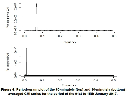
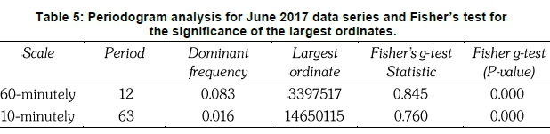
Figure 7 shows the diagrammatic representation for the largest ordinate at periods 12 and 63 for 60-minutely and 10-minutely June data series, respectively. This equates to the harmonic frequencies 2r/12 and 2r/63 for the 60-minutely and the 10-minutely time scale, respectively. Fisher's g-test statistic for the 60-minutely data series is equal to 0.845 while that of the 10-minutely data series is equal to 0.760.

 

 

At a 1% significance level, the ordinates are highly significant (since p-value=0.00) for both time scales (see Table 5).

7.3 Model building and evaluation

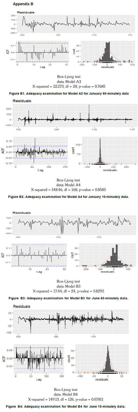
All data modelling and forecasting in this study were implemented using the R program. Sinusoidal predictor(s) were fitted using the likelihood function, such that the parameters with p-value<0.05 were deemed to be significant. The auto.arima function (from the forecast package) was used to automatically select the best SARIMA model, as illustrated in Figure 1. Parameters whose confidence band excluded zero were deemed to be significant (see Appendix A). Using the nnetar function (from the forecast package), the learning sample was preselected to be 2000, to ensure model robustness (Hyndman and Athanasopoulos, 2013). The four best-performing models were validated by examining the autocorrelation structure of the residuals using the Ljung Box test (p-value>0.05) and residual plot (mean-variance around zero) (see Appendix B).

The AIC and BIC were utilised to identify the most appropriate model amongst those fitted. In model validation, two-days-ahead forecasts were used to compare the forecasting abilities of each of the models fitted, based on performance metrics (i.e. MAE, RSME and MAPE). Smaller values of the performance metrics implied a higher accuracy level.

The prediction intervals of the forecasts from the best performing models in each of the time scales of interest were used as a measure of uncertainty in the forecasts. The confidence interval of the forecast is the band or range that is most likely to contain the mean response for the actual values of the independent variable (e.g. GHI). Prediction interval at 100(l-a)% for the value I steps ahead can be calculated by

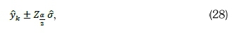
where a is the estimate of the standard deviation of the residual errors e_n(l) (see (Hyndman and Athanasopoulos, 2013)). The upper and lower limits of the confidence interval provide the optimistic and pessimistic forecasts of the independent variable.

7.3.1 Model building and selection

In neural networks, there is no specific methodology for determining the best design of the network, so the AIC and BIC results presented in Tables 6 and 7 were only calculated for the final harmonically coupled models, with the aid of the likelihood function in R software. In all the fitted models that follow, the series {W_k} denotes the non-stationary residuals (Ranganai and Nzuza, 2015).

 

7.3.1.1 Model building

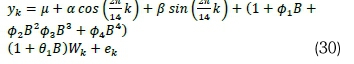
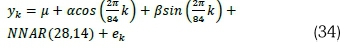
Models fitted on the 60-minutely averaged January GHI data series

• Model A1 (HCSARIMA-NNAR):

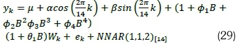
. Model A2 (HCSARIMA):

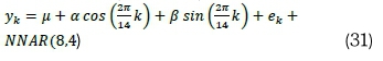
. Model A3 (HCNNAR):

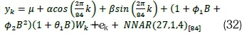
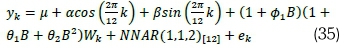
Models fitted on the 10-minutely averaged January GHI data series

• Model A4 (HCSARIMA-NNAR):

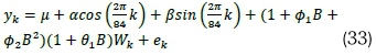
. Model A5 (HCSARIMA):

. Model A6 (HCNNAR):

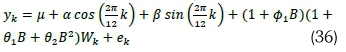
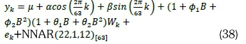
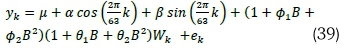
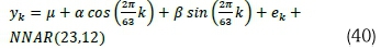
Models fitted on the 60-minutely averaged June GHI data series

. Model B1 (HCSARIMA-NNAR):

. Model B2 (HCSARIMA):

. Model B3 (HCNNAR):

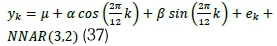
Models fitted on the 10-minutely averaged June GHI data series

• Model B4 (HCSARIMA-NNAR):

. Model B5 (HCSARIMA):

. Model B6 (HCNNAR):

7.3.1.2 Comparison of the in-sample diagnostics of the models

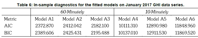
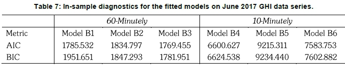
For 60-minutely averaged January data set, Model A3 was superior over Model A2 and Model A1, since it had the least values of both AIC and BIC. When compared to Model A5 and Model A6, Model A4 was superior (i.e. least values of AIC and BIC) at modelling the 10-minutely averaged January data (see Table 6). Model B3 was found to be a better (i.e. least values AIC and BIC) model than Model B2 and Model B1 at modelling the 60-minutely data series for June. The 10-minutely data series for June can be modelled better by Model B4 as it has the least values of AIC and BIC when compared to Model B5 and Model B6 (see Table 7).

7.3.2 Model evaluation

7.3.2.1 Comparison of the forecasting performance of the models

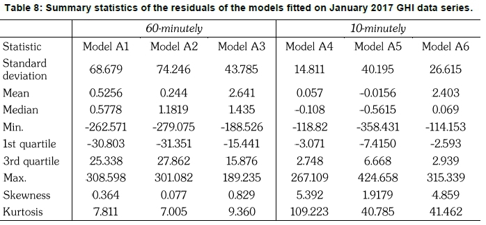
Table 8 presents the summary statistics of the residuals of the models fitted on the January 2017 GHI data series. The least values of standard deviation indicate a small variation between the forecasts and the actual GHI values. Residuals from Model A3 and Model A4 have the least standard deviation values of 43.785 and 14.811 for the 60-minutely and 10-minutely time scales, respectively. Thus, Model A3 and Model A4 are best at modelling the underlying characteristics of the January GHI 2017 data series. The positive skewness values of 0.829 and 1.918 for Model A3 and Model A4, respectively, reflect a large number of positive errors, indicating the underestimation of the January GHI data series.

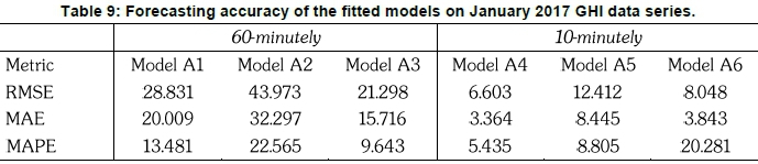
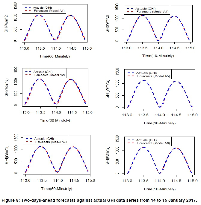
Table 9 presents the two days ahead forecasting performance of the models fitted on the 60-minutely and 10-minutely January 2017 GHI data series. For a 60-minutely time scale, the results show that Model A3 outperforms both Model A2 and Model AÍ across all error measures. For a 10-minutely averaged time scale, Model A4 consistently outperformed both Model A5 and Model A6 across all error measures. The overall results show that Model A3 and Model A4 yield the best results when forecasting 60-minutely and 10-minutely data series, respectively.

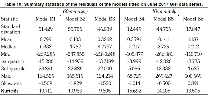
Table 10 presents the summary statistics of the residuals of the models fitted on the June 2017 GHI data series. The least values of standard deviation indicate that there is a small variation between the predicted and actual values. The least values of standard deviation were recorded for the residuals from Model B3 and Model B4 with 46.039 and 12.449 for the 60-minutely and 10-minutely time scales, respectively. These values indicate that Model B3 and Model B4 are best at modelling the underlying characteristics of the June 2017 GHI data series. Furthermore, the negative skewness values for Model B3 and Model B4 reflect a large number of negative errors, which indicate the overestimation of the GHI values.

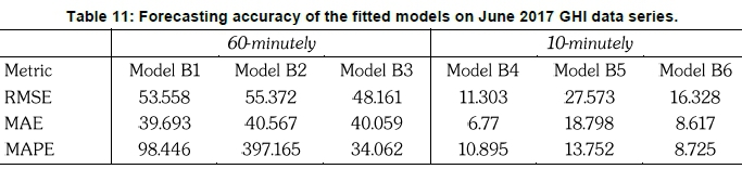
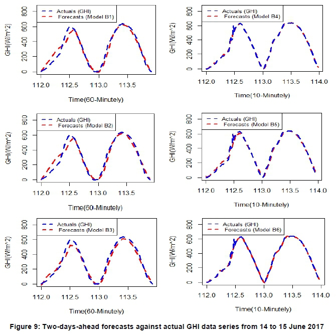
Table 11 presents the forecasting results of the models fitted on the 60-minutely and 10-minutely June 2017 GHI data series. For the 60-minutely averaged time scale, Model B3 outperforms Model B2 and Model B1 across all error measures. However, Model B1 provides better results than Model B2 across all performance metrics. On the other hand, Model B4 outperforms Model B5 across all error measures in predicting the 10-minutely time scale data. Although Model B4 is superior to Model B6 in terms of MAE and RMSE, Model B6 has a competitive edge over Model B4 in terms of MAPE. For the same time scale, Model B6 outperforms Model B5 across all error measures. The overall results show that Model B3 and Model B4 produced the best results when forecasting 60-minutely and 10-minutely data series, respectively.

Figures 8 and 9 graphically compare the two days ahead forecasts (dashed red line) against actual GHI data (blue line) from all the fitted models on the GHI data series for January and June 2017. The forecasting results showed that the predicted values fit the January 2017 data better than the June 2017 data.

7.3.2.2 Comparison of the prediction intervals

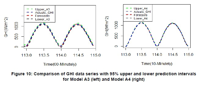
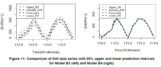
Figures 10 and 11 present the 95% prediction intervals of the forecasts from the two best models for each of the months and their respective time scales. The upper and lower limits of the prediction interval provides the optimistic and pessimistic forecasts of the GHI data. Amongst the best models (i.e. Model A3 and Model B3) for forecasting 60-minutely time scale data, the confidence bands for Model A3 were narrower than Model B3. Similarly, the prediction intervals for the best models (i.e. Model A4 and Model B4) for modelling 10-minutely time scale data were narrower for Model B4 than Model A4.

 

8. Discussion of the results

The in-sample diagnostics (i.e. AIC and BIC) results showed that HCNNAR models (i.e. Model A3 and Model B3) were superior to HCSARIMA-NNAR and HCSARIMA models in modelling larger time-scale GHI data series (i.e. 60-minutely), whilst HCSARIMA-NNAR models (i.e. Model A4 and Model B4) had a competitive edge over HCSARIMA and HCNNAR models in modelling smaller time- scale GHI data series (i.e. 10-minutely) (see Tables 6 and 7). When harmonically coupling sinusoidal predictors, only the first sinusoidal predictor was fitted on the largest ordinate of the GHI data, to minimise the values of AIC and BIC while allowing the SARIMA model to capture some of the periodicities. Besides, the inclusion of a second sinusoidal predictor had very little improvement in the forecasting accuracy.

In the forecasting arena, HCNNAR models (i.e. Model A3 and Model B3) outperformed the HCSARIMA-NNAR and HCSARIMA models in forecasting the 60-minutely time scale GHI data for each of the months of interest. For the 10-minutely time scale GHI data, the HCSARIMA-NNAR models (i.e. Model A4 and Model B4) outperformed the HCSARIMA and HCNNAR models (see Tables 9 and 11).

The HCNNAR models (i.e. Model A3 and Model B3) produced the smallest values of the standard deviation of the residuals compared to the other classes of models (i.e. HCSARIMA-NNAR and HCSARIMA) when predicting 10-minutely time-scale GHI data for each month of interest. For the 60-minutely time-scale GHI data, HCSARIMA-NNAR models (i.e. Model A4 and Model B4) outperformed HCSARIMA and HCNNAR models, as they had the least values of standard deviation for the two months under investigation (see Tables 8 and 10).

The 95% prediction intervals of the forecasts from all the best four models were valid.

However, Models A3 and Model A4 had narrower and robust prediction interval limits than Model B3 and Model B4. Thus, Model A3 and Model A4 forecasting results are more robust than Model B3 and Model B4 (see Figures 10 and 11), affirming that the predicted values fit the January 2017 data series better than June 2017 data series (see Figures 8 and 9).

 

9. Conclusions

Time-series forecasting accuracy forms a foundation for an effective decision-making process. Hence, the research towards improving the effectiveness of prediction models is of utmost importance (Zhang, 2003). This research study compared the forecasting performance of the three classes of harmonically coupled models, namely the HCSARIMA, HCNNAR and HCSARIMA-NNAR models in forecasting South African solar irradiance data. The developed forecasting models were based on the GHI data from the RVD radiometric station in the Northern Cape. The study results indicated that the HCNNAR and HCSARIMA-NNAR models were more effective at improving forecasting accuracy and handling the periodicities due to diurnal cycles, as well as the deterministic and stochastic components, than the HCSARIMA models. Restriction of sinusoidal predictors to the first predictor helped to minimise the values of AIC and BIC while improving the prediction accuracy. The in-sample and out-of-sample diagnostics results showed that HCNNAR models were best at modelling and forecasting a larger time scale (i.e. 60-minutely) whereas HCSARIMA-NNAR models were best at modelling and forecasting a smaller time scale (i.e. 10-minutely). The prediction intervals of the forecasts for the best four models (i.e. Models A3, A4, B3 and B4) were found to be satisfactory and valid. However, Model A3 and Model A4 fitted to the January data series produced narrower and robust prediction intervals. The significant contribution of this research study is in the inclusion of the NNAR models and SARIMA-NNAR models, and the combination of these models at determined harmonic frequencies to form HCNNAR models and HCSARIMA-NNAR models. The study results are compatible with some of the solar irradiance modelling studies that have applied harmon-ically coupled models to improve forecasting error (see Ranganai and Nzuza, 2015). The study will make a significant contribution to the renewable energy field, specifically short-term solar irradiance modelling. Policymakers and utility managers can use the study results to draw effective integration strategies of large volumes of solar power in the national electrical grid.

 

Author contributions

KS Sivhugwana: Research formulation, data analysis and write-up.

E Raganab Research formulation, data analysis, quality assurance and guidance in write-up.

 

References

Ahdesmaki, A., Lahdesmaki, H., and Yli-Harja, O. (2007). Robust Fisher's test for periodicity detection in noisy biological time series. IEEE International Workshop on Genomic Signal Processing and Statistics, Tuusula, 1-4. doi: 10.1109/GENSIPS.2007.4365817.         [ Links ]

Akaike, H. (1983). Information measures and model selection. Bulletin of the International Statistical Institute, 50: 277-290.         [ Links ]

Baridam, B., and Irozuru, C. (2012). The prediction of prevalence and spread of HIV/AIDS using artificial neural network: The case of Rivers State in the Niger Delta, Nigeria. International journal of Computer Applications, 44 (2): 0975-8887. https://doi:10.5120/6239-8584.         [ Links ]

Brooks, M. J., du Clou, S., van Niekerk, J. L, Gauche, M. J., Leonard, P., Mouzouris, C, Meyer, A. J., van der Westhuizen, E. E., van Dyk, N., and Vorster, F. (2015). SAURAN: A new resource for solar radiometric data in Southern Africa. Journal of Energy in Southern Africa, 26 (1): 2-10. https://doi.org/10.17159/2413-3051/2015/v26ila2208.         [ Links ]

Box, G. E. P., Jenkins, G. M., and Reinsei, G. C. (1994). Time series analysis, forecasting and control (3rd Edition). New Jersey: Prentice Hall.         [ Links ]

Box, G. E. P, and Jenkins G. M. (1976). Time series analysis: Forecasting and control. Operational Research Quarterly, 22:199-201.         [ Links ]

Bozkurt, O. O., Biricik, G., and Taysi, C. Z. (2017). Artificial neural network and SARIMA based models for power load forecasting in Turkish electricity market. PloS one, 11: e0175915. https://doi.org/10.1371/journal.pone.0175915.         [ Links ]

Chaturvedi, D. K., and Isha, I. (2016). Solar power forecasting: A review. International Journal of Computer Applications (0975 - 8887), 145: 28-50. https://doi:110.5120/ijca2016910728.         [ Links ]

Chu, Y., Urquhart, B., Gohari.S. M., Pedro, H. T., Kleissl, J., and Coimbra, C. F. (2015). Short-term reforecasting of power output from a 48 mwe solar PV plant. Solar Energy, 112: 68-77. http://dx.doi.Org/10.1016/j.solener.2014.ll.017.         [ Links ]

Diagne, H. M., David, M., Lauret, P., Boland, J., and Schmutz, N. (2013). Review of solar irradiance forecasting methods and a proposition for small-scale insular grids. Renewable and Sustainable Energy Reviews, 27: 65-76. https://doi:10.1016/j.rser.2013.06.042.         [ Links ]

Fonseca Jr., J. G. S., Oozeki, T., Takashima, T., and Ogimoto, K. (2011). Analysis of the use of support vector regression and neural networks to forecast insolation for 25 locations in Japan. In: Proceedings of ISES Solar World Congress. Kassel, Germany.         [ Links ]

Govindasamy, T. R., and Chetty, N (2019). Non-linear multivariate models for the estimation of global solar radiation received across five cities in South Africa. Journal of Energy in Southern Africa, 30 (2): 38-51. https://orcid.org/0000-0002-9809-4230.         [ Links ]

Hyndman, R. J., and Athanasopoulos, G. (2013). Forecasting: Principles and practice. Retrived from https://otexts.com.         [ Links ]

Inanlougani, A., Reddy, T. A., and Katiamula, S. (2017). Evaluation of time-series, regression and neural network models for solar forecasting: Part I: One-hour horizon, 1-20        [ Links ]

IRENA [International Renewable Energy Agency]. (2016). The power to change: Solar and wind cost reduction potential to 2025. Retrived from: https://www.irena.org/-/media/Files/IRENA/Agency/Publication/2016/IRENA_Power_to_Change_2016.pdf        [ Links ]

Khalek, A., and Ali, A. (2015). Comparative study of Wavelet-SARIMA and Wavelet- NNAR models for groundwater level in Rajshahi District. IOSR Journal of Environmental Science, Toxicology and Food Technology (IOSR-JESTFT), 10 (7): 2319-2399.         [ Links ]

Kibirige, B. (2018). Monthly average daily solar radiation simulation in: northern KwaZulu-Natal: A physical approach. South African Journal of Science, 114:1-8. https://doi.org/10.17159/sajs.2018/4452        [ Links ]

Liew, A. W.C., Law, N. F., Cao, X. Q., and Yan, H. (2009). Statistical power of Fisher test for the detection of short periodic gene expression profiles. Pattern Recognition, 42: 549-556. https://doi.Org/10.1016/j.patcog.2008.09.022        [ Links ]

Lorenz, E., Hammer, A., and Heinemann, D. (2004). Short term forecasting of solar radiation based on satellite data. In: Proceedings of EuroSun 2004 Congress. Freiburg, Germany: 841-848.         [ Links ]

Martin, A., Kourentzes, A., and Trapero, J. R. (2015). Short-term solar irradiation forecasting based on dynamic harmonic regression. Energy, 84: 289-295. https://doi.org/10.1016/j.energy.2015.02.100.         [ Links ]

Mpfumali, P., Sigauke, C, Bere, A. and Mulaudzi, S. (2019). Day ahead hourly global horizontal irradiance forecasting-application to South African data. Energies, 12(18): 1-28. https://doi.org/10.3390/enl2183569        [ Links ]

Mukaram, M. Z., and Yusof, F. (2017). Solar radiation forecast using hybrid SARIMA and ANN model: A case study at several locations in peninsular Malaysia. Malaysian Journal of Fundamental and Applied Sciences - Special Issue on Some Advances in Industrial and Applied Mathematics, 13 (4): 346-350. https://doi:10.11113/mjfas.vl3n4-1.895.         [ Links ]

Pavlovski, A., and Kostylev, V. (2011). Solar power forecasting performance towards industry standards. In: 1st International Workshop on the Integration of Solar Power into Power Systems. Aarhus, Denmark.         [ Links ]

Pretorius, P., and Sibanda, W. (2012). Artificial neural networks: A review of applications of neural networks in the modeling of HIV epidemic. International Journal of Computer Applications, 44(16): 14.         [ Links ]

Ranganai, E., and Nzuza, M. B. (2015). A comparative study of the stochastic models and harmonically coupled stochastic models in the analysis and forecasting of solar radiation data. Journal of Energy in Southern Africa, 26(1): 25-137.         [ Links ]

Schwarz, G. (1978). Estimating the dimension of a model. The Annals of Statistics, 6: 461-464.         [ Links ]

Sena, D., and Nagwani, N. K. (2016). A neural network autoregression model to forecast per capita disposable income. ARPN Journal of Engineering and Applied Sciences, 11(22): 13123-13128.         [ Links ]

Suleiman, E. A., and Adejumo, A. O. (2017). Application of ARMA-GARCH models on solar radiation for South Southern Region of Nigeria. Journal of Informatics and Mathematical Sciences, 9(2): 405-416. http://dx.doi.org/10.26713%2Fjims.v9i2.742.         [ Links ]

Voyant, C, Notton, G., Kalogirou, S., Nivet, M., Paoli, C, Motte, F., and Fouilloy, A. (2017). Machine learning methods for solar radiation forecasting: A review. Renewable Energy, 105: 569-582.         [ Links ]

Voyant, C, Muselli, M., Paoli, C, and Nivet, M. L. (2011). Optimization of an artificial neural network dedicated to the multivariate forecasting of daily global radiation. Energy, 36: 48-59.         [ Links ]

Wei, W. (2006). Time series analysis: Univariate and multivariate methods (2nd Edition). Boston: Addison-Wesley.         [ Links ]

Yarmohammadi, M. (2011). A filterbased Fisher g-test approach for periodicity detection in time series analysis. Scientific Research and Essays, 6: 7317-3723. https://doi:10.5897/SRE11.802.         [ Links ]

Zhang, G. P. (2003). Time series forecasting using a hybrid ARIMA and neural network model. Neurocomputing, 50:159-175.         [ Links ]

Zhang, J., Hodge, B. M., Florita, A., Lu, S., Hamann, H. F., and Banunarayanan, V. (2013). Metrics for Evaluating the Accuracy of Solar Power Forecasting. In: preceedings of the 3rd International Workshop on Integration of Solar Power into Power Systems. London, England.         [ Links ]

Zhandire, E (2017). Predicting clear-sky global horizontal irradiance at eight locations in South Africa using four models. Journal of Energy in Southern Africa, 28: 77-86. https://doi.org/10.17159/2413-3051/2017/v28i4a2397.         [ Links ]

 

 

* Corresponding author: 28 Pioneer Ave, Florida Park, Roodepoort, 1709; tel: +27(0)730870330; e-mail: ranganae@unisa.ac.za