ARTICLES

 

An intelligent alternating current-optimal power flow for reduction of pollutant gases with incorporation of variable generation resources

 

 

Sumant Lalljith^I; Andrew G. Swanson^I; Arman Goudarzi^{II, *}

^ISchool of Electrical, Electronics and Computer Engineering, University of KwaZulu-Natal, Howard College, Durban 4001, South Africa. https://orcid.org/0000-0003-4798-7028. ORCiDs: S. Lalljith: https://orcid.org/0000-0003-4798-7028; A.G. Swanson: https://orcid.org/0000-0002-9965-4746
^IICollege of Electrical Engineering, Zhenjiang University, Hangzhou 310000, China; School of Electrical, Electronics and Computer Engineering, Mapua University, Manila, Philippines. A. Goudarzi: https://orcid.org/0000-0003-1264-6194

 

 

---

ABSTRACT

Frequent escalations in fuel costs, environmental concerns, and the depletion of non-renewable fuel reserves have driven the power industry to significant utilisation of renewable energy resources. These resources cannot satisfy the entire system load demand because of the intermittent nature of variable generation resources (VGRs) such as wind and solar. Therefore, there is a need to optimally schedule the generating units (thermal and VGRs) to reduce the amount of fuel used and the level of emissions produced. In this study, an AC-power flow in conjunction with combined economic and environmental dispatch approach through the implementation of a modified constricted coefficient particle swarm optimisation was used to minimise the fuel cost and the level of emission gases produced. The approach was applied to the Institute of Electric and Electronic Engineers 30 bus test system through three different load conditions: base-load, increase-load and critical-load. The results showed the practicality of the proposed approach for the simultaneous reduction of the total generation cost and emission levels on a large electrical power grid while maintaining all the physical and operational constraints of the system.
HIGHLIGHTS:
• Considering several physical and environmental constraints of generating units.
• Proposing a metaheuristic method based on swarm intelligence for solving AC-OPF problem.
• Incorporation of variable generation resources in electricity spot markets.
• Maximisation of social welfare and minimisation of total generation cost, while reducing the volume of pollutant gases.

Keywords: combined economic and emission dispatch, modified constricted coefficient particle swarm optimisation, metaheuristic optimal power flow, variable generation resources

---

 

 

1. Introduction

Optimal power flow (OPF) is the result of combining economic dispatch (ED) and power flow studies [1]. The operating cost in ED is optimised by a suitable distribution of the amount of power generated by different generating units. Its primary objective is to determine the optimal redistribution of the generator power outputs to meet the load demand at the minimum operating cost, while satisfying a set of qualitative system constraints. It has become necessary to not only minimise fuel cost but also reduce the level of emissions gases, because of increased environmental concerns about thermal power plants releasing a significant level of pollutants such as mercury (Hg°), carbon dioxide (C0₂), sulphur oxides (SO_x) and nitrogen oxides (NO_x) into the atmosphere. The resulting problem is called combined economic and emission dispatch (CEED) [2]. Several methods to reduce the production of emission gases have been considered [2, 3]. The scheduling of generators, fuel cost and the transmission line characteristics of a power system network have a key influence over a generator's ability to optimise the total production cost and transmission losses. System operators are required to schedule the generating units in a manner which lowers the rate of pollutant gas production. However, this must be done together with maintaining the system security, especially in the presence of variable generation resources (VGRs).

Wind and solar power generation are the primary categories of VGRs since they are very intermittent [3]. Solar power is a renewable energy, with sunlight converted into electrical energy using solar photovoltaic (PV) technology [3]. High capital costs and the need for appropriate geographical locations are becoming increasingly minor obstacles in the application of renewable energy resources because of a promising growth of the renewable energy research and development curve [3].

Traditionally, classical optimisation techniques like lambda iteration and linear programming were used to solve the optimal power flow (OPF) problem with considerable accuracy and efficiency. However, optimisation, while maintaining an acceptable system performance, renders it impractical to solve the task using these traditional techniques [4]. There is an emerging need to integrate reliable artificial intelligence (AI) methods that can solve this complex problem efficiently. Heuristic AI optimisation methods, e.g., genetic algorithm, particle swarm optimisation (PSO), and artificial bee colony are capable of handling complex system constraints.

In this study, an OPF algorithm-based approach was used to reduce the level of emission gases produced by conventional generators with respect to the global trend towards the reduction of pollution gases. To solve the OPF problem, a modified metaheuristic algorithm based on the improved version of PSO was designed.

 

2. Methodology

An algorithm was designed to utilise a larger proportion of intermittent renewable energy that is available at any one time. This was done with consideration to various real-world power system constraints. Wind and solar PV generators were modelled for integration into the Institute of Electric and Electronic Engineers (IEEE) 30-bus test system. After a comprehensive study on different plausible heuristic AI optimisation techniques that could be used to efficiently solve the OPF problem, modified constricted coefficient particle swarm optimisation (MCCPSO) was developed. The following sub-sections explain the formulated objective function and the proposed optimisation method.

Objective functions

The OPF problem can be mathematically expressed as a series of equations starting with Equations 1 and 2.

where F(x) is the main objective function of the study; g(x) represents the set of the equality constraints; and h(x) defines the set of the inequality constraints.

Therefore, x^Tcan be expressed as Equation 3 where ng is the number of the generator, Pg_ngis the active power of the generator ng; Vg_ngis the voltage of the generator ng; T_ntis the thermal limit of the transmission line nt; and Qc_ncis the reactive power of the bus nc.

Economic dispatch objective function: The ED objective function is primarily used in the OPF problem for the minimisation of the overall cost of generation and is given by Equation 4.

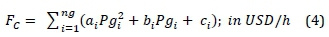
where F_cis the total generation cost function; a_i, b_i and c_iare the generators' cost coefficients; and Pg_iis the active power of the i^thgenerator.

Emission dispatch objective function: Pollutants such as SO_xand NO_xare major waste emissions into the atmosphere by thermal power plants.

The problem for minimising the quantity of emissions, E_T, is formulated by including the reduction of emissions as an objective function using Equation 5.

where E_Tis the total generator emissions function and d_i, e_i and f_i are the generators' emission coefficients. The pollution control cost, F_E(USD/h), can be obtained by assigning a cost factor to the pollution level, expressed as in Equation 6.

where h_m is emission control cost factor and represents the ratio of the maximum fuel cost to the minimum emissions of the generating units [2], as in Equation 7.

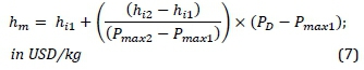
where h_i2 and h_irare price penalty factors associated with the last and the current unit; P_max2 and P_max1are the maximum powers associated with the last and the current unit; and P_Dis the power demand of the system. Therefore, the price penalty factor of the i^thunit (h) can be calculated using Equation 8.

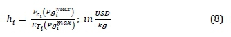
where F_cis the generation cost of the i^thunit and E_T. is the emission volume of the i^thunit.

The CEED objective function: The ED minimises the total operating cost at the expense of increasing the rate of emission gases such as N0_X. On the contrary, emission dispatch minimises the volume of emission gases released by the system at the expense of an increased system operating cost. In this study, the operating and emission cost simultaneously was reduced mathematically as in Equation 9.

subject to the load demand equality and the generator inequality constraints.

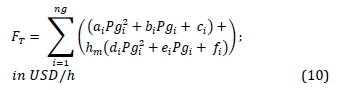
A multi-dimensional optimisation is converted into a single-dimensional optimisation problem by introducing the price penalty factor, h_m, in Equation 10.

The equality constraints: The i^thbus injected active and reactive powers are described using equality constraints and can be defined by Equation 11 [5].

where P_lossesis the total generation loss.

The inequality constraints: The inequality constraints associated with the power system network represent the physical limits of the components. These constraints ensure maintenance of the system security [5]. Equations 12-15 represent the inequality constraints of the control variables considered in this study.

where Pg_i,min and Pg_i,maxare the minimum and the maximum active generation capacity of the i^th generator; Qg_i,min and Qg_i,maxare the minimum reactive generation capacity of the i^thgenerator; MVAf_p,qis the transmission line power flow constraint between bus q and bus p; MVAf^max_p,qis the maximum power that can flow between bus q and bus p; and V_i,min and V_i,maxare the minimum and the maximum voltage of the i^thP-Q bus constraint.

2.2 Variable generation resources

Wind power generation: The wind speed gained by the wind turbines is usually effective at 50-100 m above ground [6]. Thus, the wind speed measured by the anemometer (at its height above ground) needs to be converted to the turbine's hub height [7]. Equation 16 explains the relationship of the wind speeds at different height hubs.

where v₁ and v₂are the wind speed at the initial and the changed hub height respectively; h₁ and h₂ are the hub height of the initial and selected point respectively; and a is the friction coefficient that implicates actual parameters such as the roughness of terrain and temperature. The power generated from the wind turbine can be approximated by Equation 17 [7] (see foot of page).

The cost of wind power generation: The total cost of power production from the wind farm can be calculated using Equation 18 [8, 9] (see foot of page).

The solar PV power generation: Solar PV power is reliant on natural occurrences such as solar irradiance and the ambient temperature. These quantities are directly related to geographical location and season. The power generated from a solar PV farm is calculated by Equation 19 [10, 11].

For a given radiation level and ambient temperature, the voltage-current characteristics of a PV module are determined using Equations 20-23.

where P₀(s) is the power generated by the solar farm; s is the solar irradiance; N is the number of the PV modules; FF is the fill factor of the PV module; Vp_Vis the voltage of the PV module; I_PVis the current of the PV module; V_MPPTis the voltage of the maximum power point tracking of the PV module; I_mpptis the current of the maximum power point tracking of the PV module; V_ocis the open-circuit voltage of the PV module; I_scis the short-circuit current of the PV module; K_vis the voltage temperature coefficient; T_PVis the PV cell temperature; K_tis the current temperature coefficient; and V_ocis the open-circuit voltage.

The cost of solar PV generation: The total cost of power production from the solar PV farm can be calculated using a cost function represented by Equation 24 [12] (see foot of page).

The penalty cost coefficient is caused by not using all the available wind/ solar PV power available. It is the difference between the available wind power and the actual wind power used. The reserve cost coefficient is caused by under-generation; hence this coefficient is associated with the calling of reserves for compensation [9]

where P_windis the power generated by the wind turbine; V is the wind speed, V_cut__inis the cut-in wind speed of the wind turbine; V_cut__outis the cut-out speed of the wind turbine; V_ris the rated speed of the wind turbine; and P_ris the rated power wind turbine.

where C_w. is the total cost of the generated power by the i^thwind farm; w_iis the total generated power by the i^thwind farm; d_i(w_i) is the direct cost of wind power; k_pi(w_i) is the penalty cost coefficient for overestimation of the wind power; and k_ri(w_t) is the reserve cost for the underestimation of the wind power.

where C_s. is the total cost of the generated power by the i^thsolar farm, S_tis the total generated power by the i^thsolar farm, d_i(S_i) is the direct cost of solar power, k_pi(S_i) is the penalty cost coefficient for overestimation of the solar power; and k_ri (S_t) is the reserve cost for the underestimation of the solar power.

2.3 Formulation of the MCCPSO-OPF

Load flow methodology: In an electrical grid, power flows from the generation stations to the load centres. Thus, an investigation is required to determine the bus voltages and the power flow through the transmission lines. There are many methods (such as Newton-Raphson (NR), Gauss-Siedel, or Fast-Decoupled [13]) that can be used to perform the load flow calculations, however, to ensure that the system performs at an optimal level a load flow method needs to be selected based on merit and practicality. The NR method was selected because of its mathematical superiority and accuracy [14-17].

2.4 A modified constriction coefficient PSO

The PSO is a population-based stochastic optimisation technique developed in 1995 and inspired by the social behaviour of birds flocking and fish schooling [18]. In other words, its development was based on the behavioural ability of the swarms to share their information with each other (information is what food sources, danger, etc, are referred to as), where this characteristic increases the efficiency of the entire swarms as opposed to individual particle exploration.

The PSO contains a population of candidate solutions (randomly generated on the first iteration) called a swarm. In every iteration, every particle is a candidate solution to the optimisation problem, in which every particle has a position in the search space. Consider the particle having a position and velocity as stated in Equations 25 and 26.

For particle i,

Figure 1 shows a simple model of a moving particle in PSO, one which is not alone but part of a swarm. A particle (x_l(t)) moves towards the optimum solution based on its present velocity (v_l(t)), its previous experience (stored in memory) and the experience of its neighbours. In addition to the position and velocity of the particle, every particle has a memory of its own best position. This is denoted by P_L(t), which represents the personal best experience of the particle. In addition to P_L(t), there is a common best experience among the members of the swarm. This is denoted by G (t) (this is not denoted by i, as it belongs to the entire swarm and not just to the particle), which represents the global best experience of all the particles in the swarm.

The mathematical model of PSO is simple. By defining these concepts on every iteration of PSO the position and velocity of the particle are updated according to the best experience. Figure 1 defines a vector from the current position to the personal best solution and a vector from the current position to the global best. The particle tends to move towards the new position using all the vectors shown. The black line indicates the motion of the vector as it moves to the new position (denoted by x_i(t + 1) ). The new velocity is denoted by v_l(t + 1). A new position is created according to the previous velocity v_i(t), the personal best P_L(t), and the global best G(t). Therefore, x_i(t + 1) is probably a better location (solution) as the particle was guided by its own motion (its memory of the previous best experience and the experience of the entire swarm). The velocity and position of each particle can be calculated using Equations 27 and 28 (see top of next page).

In the velocity updating process, the values of parameters such as c₁and c₂are equal to 2.05. The r₁and r₂generate random numbers between 0 and 1. Equations 26 and 27 represent the basic version of the PSO algorithm, but several modifications are necessary to enhance the performance of the PSO.

Thus, this study has proposed the following methods to modify the basic PSO:

Modification #1: In order to enhance the functionality of the random components' coefficients of the vector of velocity (r₁and r₂), they should generate the random numbers according to the size of the variable matrix and the produced values should be subtracted from 1. Therefore, Equation 27 can be modified as Equation 29 (see top of page)

Modification #2: The vector of velocity should go under a refinement process once its values are defined through the Equation 29, to further improve its performance, as shown in Equations 30 and 31.

where

where Vel_maxis the maximum range of the vector of the velocity at that step; and Var_maxand Var_min are the maximum and minimum values for the size of the variables.

Modification #3: In this formulation, the study has implemented a constriction coefficient method to precisely determine the values of the velocity coefficient (c₁and c₂). The amplitude of a particle oscillations decreases as it focuses on the local and neighbourhood previous best positions. Through this method, the movement of particles will be confined to optimum point over time, also it prevents the particles from trapping in local minima [17]. The third modification for improving the performance of PSO can be implemented through Equations 32-35.

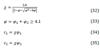
where x is the constriction coefficient; k is the constant multiplier in the constriction coefficient technique (typically, the value of k is between 0.73 to 1); φ is the convergence factor; c₁is the fixed coefficient for the personal best experience and c₂ is the fixed coefficient for the global best experience.

Modification #4: To create a suitable balance between the exploration and exploitation during the optimisation process, the study proposed a non-linear time-varying damping inertia (NLTVD) technique. The NLTVD dynamically reduces the value of damping inertia from its maximum value towards its lower bound as the optimisation progresses. Also, it prevents the PSO from any premature convergence. (See Equations 36 and 37 below.)

where w^Max and W^Minare the maximum (0.9) and minimum (0.4) values for the damping inertia coefficient; a₁and a₂are multiplicative coefficients of NLTVD, where the value of a₁is 0.2 and the value of a₂is 7; Iter_iis the current iteration; and Max_Iteris the maximum number of iterations.

where Pop_numberis the population number; and rand_igenerates random integers according to population number and size of the variables.

Modification #5: To reduce the destructive impact of the weak particles, a crossover operator is implemented. The proposed crossover operator diversifies the populations in each iteration and it avoids the re-exploration of the inappropriate zones. (See Equation 38 at top of page.)

2.5 System overview

Application of MCCPSO in OPF: Using Equation 10, the objective function implemented in MCCPSO is defined in Equation 39.

Therefore, the constrained optimisation problem is converted into an unconstrained problem using the price penalty factor method (Equation 8). The MCCPSO algorithm in Equation 39 deals directly with the real power constraint. The application of the MCCPSO algorithm is shown in Figure 2.

After the MCCPSO algorithm determined the global optimum solution for the CEED objective function, the line-flow power in megavolt amperes (MVA) was calculated for the entire network. If the calculated line-flow power (MVA) exceeded the rated line-flow MVA, then the algorithm selects the previous G(t) value as the global optimum solution to the problem. This procedure prevents the transmission lines from being overloaded.

Newton-Raphson power flow solution: The test system data is taken from Sadaat [13]. The bus data (admittance bus, denoted by Y_bus) is used to obtain the load flow solution for the intelligent AC-OPF. The MCCPSO-OPF updates the generated power column of the bus data matrix, which indicates the power required to be generated by each generator in the system. The losses in the system are calculated only at the end of the iteration. The difference in power injection and power demand is the loss of the system. This extra power must be accommodated in the load flow for the next iteration. Hence the slack bus, being the generator bus with the highest generating capacity, accepts this extra burden to balance the system. Therefore, at this bus, the voltage magnitude and phase angle are specified, and the real and reactive powers are calculated. Figure 3 depicts the process of power flow analysis with the help of MCCPSO.

Wind power model: Three wind farms will be integrated into the IEEE 30-bus network and are modelled with respect to wind farm projects in South Africa [20] as indicated in Table 1. The total installed capacity of these wind farms was 56.7 MW. By means of the input parameters presented in Table 1, it was possible to model the wind farms for this study using Equations 18 and 19. For the best practical results, using the average wind speed data (approximately 7 m/s) gathered from the actual wind farm locations [24], an artificial wind speed simulator was developed in MATLAB R2018a.

Solar PV power model: For the integration of solar PV energy into this study, a 10 MW PV generator was considered. Solar irradiance and the ambient temperature data collected by the University of KwaZulu-Natal [25] was utilised for this model. Table 2 indicates the solar panel parameters. Following the design of a 5 MW solar PV farm [26], which used 22560 PV modules to produce this output power capacity, it takes 45 455 solar PV modules to produce 10 MW.

 

 

System integration: Considering the single-line diagram of the IEEE 30-bus network in Sadaat [13], the cookhouse, Gouda and Enel's Gibson Bay wind farms were strategically placed at buses 30, 29, and 24 respectively. The solar PV farm (10 MW) was placed at bus 23. Figure 4 illustrates a simple schematic of the overall power system network after integration.

 

 

One of the main objectives of this study was to create a control system that intelligently utilises a larger proportion of variable renewable energy when available to supply the load demand. The MCCPSO algorithm was designed to carry out this operation. The system algorithm first considered the amount of renewable power available at each hour to supply the load demand, the remainder of the load demand was then allocated to the conventional generators in the system. Equation 40 defines this operation.

where p_D^Newis the new load demand of the system; P_sis total generated power by the solar farm; and P_wis the total generated power by the wind farm.

 

3. Results and discussion

The system designed and simulated on MATLAB was executed on Inter ® Core^TM i5-7200U (2.7 GHz), 4.00 GB RAM (DDR5) and windows 10 OS (personal property). First, this section defines the main contributions of this study:

i) The proposed MCCPSO was employed to solve the OPF problem using the CEED objective function.

ii) Three wind farms were modelled on the basis of a novel algorithm formulated to artificially convert the generated wind speed variations to the power output of WTGs.

iii) A novel mathematical formulation was proposed to model the power output of mono-crystalline PV-arrays. iv) The proposed MCCPSO algorithm was implemented to intelligently utilise a large proportion of VGRs to meet the load demand at the specified hour.

v) A proposed metaheuristic OPF approach was able to maximise the social welfare, while minimise the volume of the produced pollutant gases.

3.1 The MCCPSO-OPF on the Original IEEE 30-bus

The original IEEE 30-bus test network specifications are shown in Table 3 [27, 28].

 

 

Table 4 indicates the resultant IEEE 30-bus fuel cost after applying the MCCPSO algorithm through ED and presents the potential of the proposed AI algorithm by comparing it with other AI optimisation algorithms under similar circumstances.

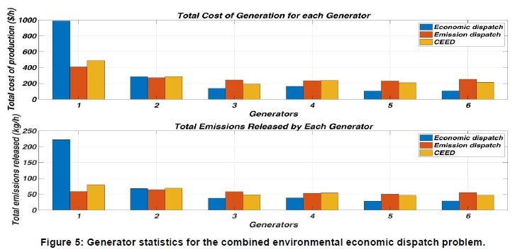
Table 5 indicates the new rate of emission gases produced through MCCPSO-OPF using the different objective functions. Although the level of emissions produced is slightly higher than what was achieved through emission dispatch, the total cost of production is significantly less; thus, an appropriate balance between the fuel cost and the level of emission gases has been established. Considering the initial fuel cost and rate of emission gases emitted, through the proposed CEED function there were 7.67% and 27% reductions in USDfh and kg/h respectively. This remarkable outcome can be attributed to the fact that dispatching the cheapest generators in a power system to meet the load demand cannot guarantee the optimum cost of operation as it can increase the power losses with respect to the geographical location of the generators and loads. The total cost of generation and the emissions released by each generating unit are shown respectively in Figures 5 and 6.

 

 

Use of the CEED objective function resulted in the dispatched power being more economical than the ED objective function, which overburdened the slack bus to optimise the fuel cost as depicted in Figure 5. Overloading of the slack bus to minimise the fuel cost resulted in a significant increase in the rate of emissions released by the slack bus alone, affecting the overall cost of production as shown in Figure 5. Overloading of the slack bus is a common issue in economic load dispatch, however, several methods to distribute this burden were studied by Panda [29].

3.2 Wind generator model

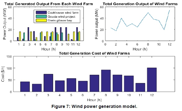
The wind speed generator was simulated to investigate the severe restrictions of the wind turbine for each wind farm. Figure 6 shows the wind speed characteristics at the selected wind farms. Figure 7 shows the power generated by each wind farm and the combined generated power. The model was developed over 12 hours, but was extended to 24 hours when integrated. The energy produced by wind farms was directly proportional to wind speed variations. The total cost of wind power generation for each hour is also indicated in Figure 7.

3.3 Solar PV generator model

In general, the temperature and irradiance levels peak between 11:00 and 15:00 pm when the sun's intensity is brightest, hence maximum power output can be expected from the PV farm during this period. The amount of solar irradiance present directly affects the amount of power produced by the 10 MW farm, as shown in Figure 8.

 

 

On every execution of the PV model over 24 hours, the results produced are dependent on the sample of seasonal data collected from [25]. As the amount of power generated by the PV model increases, so does the cost of production (USD/h). The model generally produced the best distribution of power output during the day in summer (based on an average summer day).

3.4 Generator cost comparison

The cost of power generation for the wind and solar generators were calculated using Equations 18 and 24, respectively. Table 6 shows the cost coefficients.

Table 7 shows the cost of generation per MW for each generator. Power generation from the PV farm was slightly more than wind power at 2.23 USD/MW. However, this was still better than the power produced by conventional generators. The cost of power generation by Solar PV is generally more expensive compared with wind turbine generators [30].

3.5 Integrated system model

To have a comprehensive investigation of the proposed method, the three following load conditions were considered over 24-hour cycle:

• base-load condition, 283.4 MW;

• increased load condition, 370 MW; and

• critical load condition, 160 MW.

This section presents the outcome of integrating the intermittent renewable generators into the IEEE 30-bus network under the control of the MCCPSO algorithm. Figure 9 represents the proportional contribution of the wind, solar PV, and conventional generators of the system towards the overall load demand and the total cost of generation (for each hour). It is significant to mention that, in all the presented tables in section 3.5, C_i, W_i and S_i are representing the conventional generators, wind farms and solar farms, respectively.

Figure 9 indicates the varying of the load demand conditions where a, b, and c respectively represent the baseload, increased load, and critical load conditions. The load demand conditions were programmed to consistently alternate over the 24 hours for the sake of analysis, given the intermittent nature of renewable energies. Under each load condition, for the first hour, the renewable generators were purposely omitted to investigate the effectiveness of the proposed algorithm on the test system.

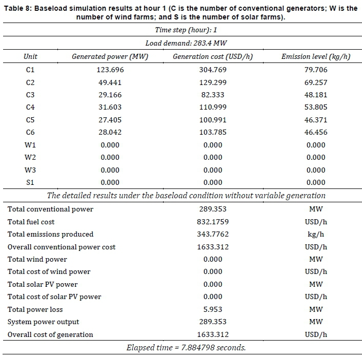
Baseload condition

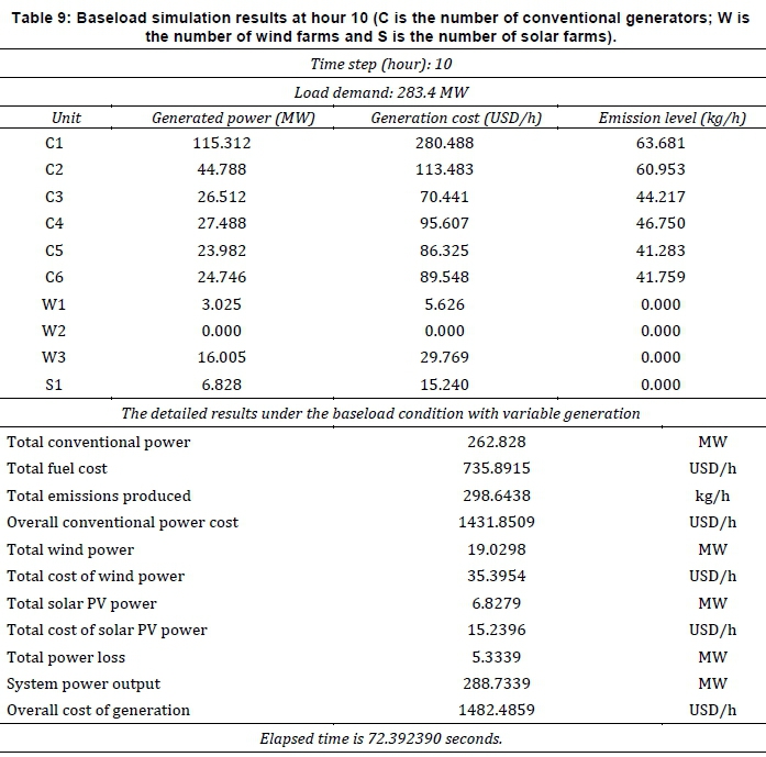
The total standard load demand of the IEEE 30-bus network was taken as 283.4 MW, which represented the baseload condition. The simulation produced the optimal dispatching of each generator for every hour through a very detailed cost analysis. Table 8 presents the optimal dispatching of the generators in the standard 30-bus network to meet the baseload demand (1^st hour). The outcome was similar to the CEED results presented in the system analysis before integrating the renewable generators (decimal variation caused by the stochastic nature of MCCPSO). Table 9 shows the dispatching of the generators in the network considering renewable power penetration (10^th hour).

Figure 10 shows the proportional power generation at the baseload demand with a reduced production cost because of the integration of renewable generators. Figure 11 indicates the produced emission volume versus power losses, where the level of emissions produced was significantly reduced after the system utilised a more significant proportion of available renewable power to meet the baseload demand.

 

 

 

 

Increased load condition

To illustrate the efficiency of the proposed algorithm, the load demand was increased to 370 MW. Table 10 represents the second hour of the simulation, which presents the outcome of introducing the increased load demand, while omitting any renewable energy penetration. Table 11 represents the system with the renewable generators contributing towards the load demand. The system algorithm efficiently dispatched all the conventional generators to meet this load demand without exceeding any of the generator constraints (evident for the real powers of generators C4 and C5 in both Tables 10 and 12, respectively) and concerning the availability of renewable energies. The proportional contribution of each generator type towards the increased load demand is shown in Figure 12. There was an increase in the cost of production, level of emissions, and the power loss as shown in Figures 12 and 13, respectively. However, with the incorporation of renewable energies, these quantities were significantly reduced. The renewable generators significantly mitigated the level of emissions produced.

 

 

Critical load condition

To test the efficiency of the proposed algorithm at the extremum points, the load demand was reduced to 160 MW. This situation is termed as the critical load condition as it is the initial point where the systems lower bound constraints might be infringed upon. Table 12 displays the outcome of the simulation without the output of renewable generators.

Table 13 shows the outcome of the simulation with renewable energies penetration. The MCCPSO algorithm efficiently dispatched each generator without infringing on the inequality constraints of the conventional generators, while taking into consideration the available renewable power.

The proportional contribution of each generator type towards the critical load demand is illustrated in Figure 14. A decrease was recorded in the cost of production, the level of emissions produced and the amount of power loss incurred, as shown in Figures 14 and 15.

 

4. Conclusions

In this study, an intelligent AC-optimal power flow (AC-OPF) through the adoption of modified constriction coefficient particle swarm optimisation (MCCPSO) was proposed for solving the dynamic power flow analysis in the presence of variable generation resources (VGRs). The proposed MCCPSO-OPF was designed to interactively incorporate a larger proportion of power supplied by VGRs into the network at any given time, considering the system security. The MCCPSO-OPF has the unique capability to comprehend and adhere to the physical and systematic operational constraints. The developed MCCPSO-OPF significantly reduced the operation cost and the emission volume by 7.67% and 27%, respectively, for a 24-hour cycle. With respect to the investigated case studies, it can be concluded that the proposed method of the study is able to maximise the social welfare, while minimising the generation costs. It can, therefore, be used by system operators in the power market industry.

 

Acknowledgements

This work has been supported by the international post-doctoral exchange fellowship programme (Talent-Introduction Program) of the People's Republic of China (Fund No. 207689). Also, the authors would like to sincerely thank the JESA editor (Dr Mok Roberts) for his professional suggestions towards uplifting the technical quality of this research.

Author roles

Sumant Lalljith: Formulation of research, computer simulation and execution, data analysis and write-up. Andrew G. Swanson: Manuscript review, data collection, supervision, technical and quality assurance. Arman Goudarzi: Hatched the initial research idea; problem formulation, supervision, computer simulation and write-up.

 

References

[1] Goudarzi, A., Li, Y., & Xiang, J. 2020. A hybrid non-linear time-varying double-weighted particle swarm optimization for solving non-convex combined environmental economic dispatch problem. Applied Soft Computing, 86, 105894. https://doi.org/10.10167j.asoc.2019.105894.         [ Links ]

[2] Goudarzi, A., Swanson, A. G., Tooryan, F., & Ahmadi, A. 2017. Non-convex optimization of combined environmental economic dispatch through the third version of the cultural algorithm. IEEE Texas Power and Energy Conference. https://doi.org/10.1109/tpec.2017.7868281.         [ Links ]

[3] Blumsack, S. 2018. Variable energy resources and three economic challenges. The Pennsylvania State University. [Online]. Available: https://www.e-education.psu.edu/eme801/node/539. [Accessed 16 July 2018].         [ Links ]

[4] Goudarzi, A., Viray, Z. N. C., Siano, P., Swanson, A. G., Coller, J. V., & Kazemi, M. 2017. A probabilistic determination of required reserve levels in an energy and reserve co-optimized electricity market with variable generation. Energy, 130, 258-275. https://doi.org/10.1016/j.energy.2017.04.145.         [ Links ]

[5] Velaga, S. & Padma, k. 2013. Combined economic and emission dispatch using multi-objective particle swarm optimization with svc installation. International Journal of Advanced Computer Research, 3(11): 13 - 18. https://doi.org/10.1.1.405.9669.         [ Links ]

[6] Monteiro, C., Bessa, R., Miranda, V., Botterud, A., Wang. J., & Conzelmann, G. 2009. Wind power forecasting: state-of-the-art. Decision and Information Services Division, Argonne National Laboratory. 1 - 216. https://doi.org/10.2172/968212.         [ Links ]

[7] Borhanazad, H., Mekhilef, S., Gounder Ganapathy, V., Modiri-Delshad, M., & Mirtaheri, A. 2014. Optimization of micro-grid system using mopso. Renewable Energy, 71, 295-306. https://doi.org/10.1016/j.renene.2014.05.006.         [ Links ]

[8] Makhloufi, S., Mekhaldi, A., Teguar, M., Koussa, D.S. & Djoudi, A. 2013. Optimal power flow solution including wind power generation into isolated adrar power system using psogsa, Revue des Energies Renouvelables, 16(4): 721 - 732. https://www.semanticscholar.org/.         [ Links ]

[9] Abuella, M. A. & Hatziadoniu, C. J. 2015. The economic dispatch for integrated wind power systems using particle swarm optimization. IEEE Conference in Charlotte, 1 - 6. https://arxiv.org/pdf/1509.01693.         [ Links ]

[10] Suresh, V. & Suresh, S. 2015. Economic dispatch and cost analysis on a power system network interconnected with solar farm. International Journal of Renewable Energy Research, 5(4):1099 - 1105. https://www.ijrer.org/.         [ Links ]

[11] ElDesouky, A. A. 2013. Security and stochastic economic dispatch of power system including wind and solar resources with environmental consideration. International Journal of Renewable Energy Research, 3(4): 951 -958. https://www.ijrer.org/.         [ Links ]

[12] Saxena, N., & Ganguli, S. 2015. Solar and wind power estimation and economic load dispatch using firefly algorithm. Procedia Computer Science, 70, 688-700. https://doi.org/10.1016/j.procs.2015.10.106.         [ Links ]

[13] Saadat, H. 1999. Power System Analysis. New York, WCB/McGraw-Hill. https://www.mheducation.com/.         [ Links ]

[14] Sereeter, B., Vuik, C., & Witteveen, C. 2019. On a comparison of Newton-Raphson solvers for power flow problems. Journal of Computational and Applied Mathematics, 360, 157-169. https://doi.org/10.1016/j.cam.2019.04.007.         [ Links ]

[15] Aslam, M. U., Cheema, M. U., Samran, M., & Cheema, M. B. 2014. Optimal power flow based upon genetic algorithm deploying optimum mutation and elitism. The 1st International Conference on Information Technology, Computer, and Electrical Engineering. https://doi.org/10.1109/icitacee.2014.7065767.         [ Links ]

[16] Goudarzi, A., Ahmadi, A., Swanson, A. G., & Van Coller, J. 2016. Non-convex optimisation of combined environmental economic dispatch through cultural algorithm with the consideration of the physical constraints of generating units and price penalty factors. SAIEE Africa Research Journal, 107(3), 146-166. https://doi.org/10.23919/saiee.2016.8532239.         [ Links ]

[17] Pranava, G., & Prasad, P. V. 2013. Constriction coefficient particle swarm optimization for economic load dispatch with valve point loading effects. International Conference on Power, Energy and Control. https://doi.org/10.1109/icpec.2013.6527680.         [ Links ]

[18] Fahad, S., Mahdi, A. J., Tang, W. H., Huang, K., & Liu, Y. 2018. Particle swarm optimization based dc-link voltage control for two stage grid connected pv inverter. International Conference on Power System Technology. https://doi.org/10.1109/powercon.2018.8602128.         [ Links ]

[19] Gharib, A., Benhra, J. & Chaouqi, M. 2018. A performance comparison of genetic algorithm and particle swarm optimization applied to tsp. International Journal of Recent Trends in Engineering and Research, 4(4), 529-536. https://doi.org/10.23883/ijrter.2018.4270.s3bvz.         [ Links ]

[20] Caboz, J. 2018. These are the 5 biggest green energy projects in SA - all wind farms. Business Inside. [Online]. Available: https://www.businessinsider.co.za/5-massive-new-renewable-energy-projects-that-transformed-south-africas-landscape-2018-4. [Accessed 7 September 2018].         [ Links ]

[21] Suzlon Energy Limited. Suzlon powering a greener tomorrow. classic fleet, [Online]. Available: https://www.suzlon.com/in-en/energy-solutions/classic-fleet-wind-turbines. [Accessed 17 September 2018].         [ Links ]

[22] The Nordex Group. AW3000 - Nordex. [Online]. Available: http://www.nordex-online.com/fileadmin/MEDIA/AW/AW3000_oct17_EU-EN.pdf&ved=2ahUKEwiVhJCIyffdAhUDXsAKHQfzCvMQFjAAegQIAhAB&usg=AOvVaw0oLQyNN65v-IWmyamss9Kz. [Accessed 8 September 2018].         [ Links ]

[23] The Nordex Group. Nordex: N117/3000. [Online]. Available: www.nordex-online.com/en/produkte-service/wind-turbines/n117-30-mw.html. [Accessed 8 September 2018].         [ Links ]

[24] South African Wind Energy Association. Wind energy. [Online]. Available: www.sawea.org.za. [Accessed 10 September 2018].         [ Links ]

[25] Southern African Universities Radiometric Network. Solar radiometric data for the public sauran, Durban. http://www.sauran.net/ShowStation.aspx?station=2.         [ Links ]

[26] Aryal, A., & Bhattarai, N. 2018. Modelling and simulation of 115.2 kwp grid-connected solar pv system using pvsyst. Kathford Journal of Engineering and Management, 1(1), 31-34. https://doi.org/10.3126/kjem.v1i1.22020.         [ Links ]

[27] Oubbati, Y., Mohammed, A. & Arif, S. 2016. Improved pso applied to the optimal power flow with transient stability constraints. Journal of Electrical Systems, 12(4): 672 - 686. https://creativecommons.org/licenses/by-nc/4.0/.         [ Links ]

[28] Reddy, S. S., & Momoh, J. A. 2016. Minimum emission dispatch in an integrated thermal and wind energy conservation system using self-adaptive differential evolution. IEEE PES Power Africa. https://doi.org/10.1109/powerafrica.2016.7556615.         [ Links ]

[29] Panda, S.R. 2013. Distributed slack bus model for qualitative economic load dispatch. National Institute of Technology, Rourkela, 1 - 45. https://www.semanticscholar.org/.         [ Links ]

[30] Augusteen, W. A., Geetha, S., & Rengaraj, R. 2016. Economic dispatch incorporation solar energy using particle swarm optimization. 3rd International Conference on Electrical Energy Systems. https://doi.org/10.1109/icees.2016.7510618.         [ Links ]

[31] Garnham, B. L. 2016. Mercury emissions from South Africa's coal-fired power stations. Clean Air Journal, 26(2), 14-20. https://doi.org/10.17159/2410-972x/2016/v26n2a8.         [ Links ]

 

 

* Corresponding author: Tel: 008613777894042. email: agoudarzi@zju.edu.cn