WINDAC 2018 CONFERENCE PAPER - NOT PEER-REVIEWED
doi: https://dx.doi.org/10.17159/2413-3051/2019/v30i2a6316

 

Clustering of wind resource data for the South African renewable energy development zones

 

 

Chantelle Y. Janse van Vuuren^{I, *} ; Hendrik J. Vermeulen^II

^IDepartment of Electrical/Electronic Engineering, Stellenbosch University, Private Bag X1, Matieland 7602, South Africa. https://orcid.org/0000-0001-8000-3583
^IIDepartment of Electrical/Electronic Engineering, Stellenbosch University, Private Bag X1, Matieland 7602, South Africa. https://orcid.org/0000-0003-4356-4044

 

 

---

ABSTRACT

This study investigates the use of clustering methodologies as a means of reducing spatio-temporal wind speed data into statistically representative classes of temporal profiles for further processing and interpretation. The clustering methodologies are applied to the high-resolution spatio-temporal, meso-scale renewable energy resource dataset produced for Southern Africa by the Council of Scientific and Industrial Research. This large dataset incorporates thousands of coordinates and represents a challenge from a computational perspective. This dataset can be reduced by applying clustering techniques to classify the temporal wind speed profiles into categories with similar statistical properties. Various clustering algorithms are considered, with the view to compare the performances of these algorithms for large wind resource datasets, namely k-means, partitioning around medoids, the clustering large applications algorithm, agglomerative clustering, the divisive analysis algorithm and fuzzy c-means clustering. Two distance measures are considered, namely the Euclidean distance and Pearson correlation distance. The validation metrics evaluated in the investigation includes the silhouette coefficient, the Calinski-Harabasz index and the Dunn index. Case study results are presented for the Komsberg Renewable Energy Development Zone, located in Western Cape, South Africa. This zone is selected based on the high mean wind speed and large standard deviation exhibited by the temporal wind speed profiles associated with the zone. The effects of seasonal variation in the temporal wind speed profiles are considered by partitioning the input dataset in accordance with the low and high demand seasons defined by the Megaflex Time of Use tariff. The clustered wind resource maps produced by the proposed methodology represent a valuable input dataset for further studies such as siting and the optimal geographical allocation of wind generation capacity to reduce the variability and ramping effects that are inherent to wind energy.

Keywords: wind energy resources, wind maps, clustering

---

 

 

1. Introduction

Wind and solar photovoltaic energy sources are not dispatchable and exhibit a high degree of variability. Flat feed-in tariffs, furthermore, encourage independent power producers to concentrate renewable energy plants in highly localised geographical regions, in order to maximise the cumulative annual energy yield. This increases the temporal variability of the cumulative renewable energy generation profile and the associated residual load profile, which increases the operational and maintenance costs associated with the conventional generation fleet. This is due to higher spinning reserve margins, increased ramp rates and generation constraints [1]. In the context of long-term planning, for high penetration of renewable energy, it is important to site wind farms such that the variability of the aggregated wind power generation profile is minimised. This can be achieved through careful consideration of the temporal characteristics of the wind speed profiles associated with potential geographical target zones.

The Council of Scientific and Industrial Research (CSIR), as part of phase two of the Strategic Environmental Assessment (SEA) study for the effective and efficient roll-out of large-scale wind and solar development in South Africa, identified eight renewable energy development zones (REDZ) to be targeted by future renewable energy developments [2]. In this context, the historical wind resource data for the REDZ regions represent an important strategic input for informed siting of wind farms in order to minimise residual load.

Medium- and long-term planning for the incorporation of wind energy resources in the energy mix generally makes use of wind atlas datasets derived by modelling approaches such as the numerical weather prediction and weather research and forecasting tools [3]. These models typically deliver datasets of mesoscale spatio-temporal wind speed profiles with given spatial and temporal resolutions. A small spatial and/or short temporal resolution gives rise to a large dataset, which is computationally intensive for modelling and interpreting the underlying spatial and temporal characteristics. Machine learning data reduction and classification methodologies, such as clustering, represents a useful tool for transforming such a large, diverse dataset into a more informative resource.

 

2. South African wind and solar resource dataset

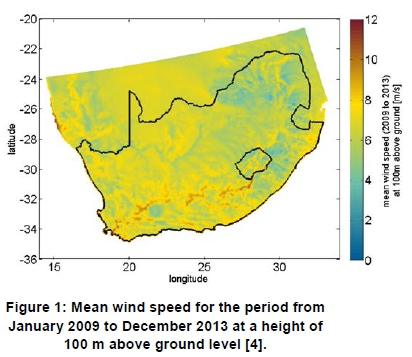
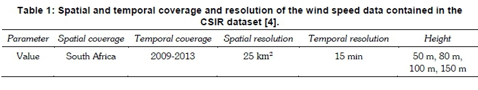
Table 1 summarises the main characteristics of the wind and solar resource dataset used in this study [4]. The dataset, which incorporates both wind and solar resource data for the whole of Southern Africa, has a spatial resolution of 5 km by 5 km and a temporal resolution of 15 minutes. The wind speed data is given for various heights, i.e. 50 m, 80 m, 100 m and 150 m above ground level. The wind speed data at a height of 100 m is used in this study, as 100 m is a standard wind turbine hub height. Figure 1 shows a spatial map of the mean wind speed at a height of 100 m for the period from January 2009 to December 2013.

 

 

2.1 Renewable energy development zones

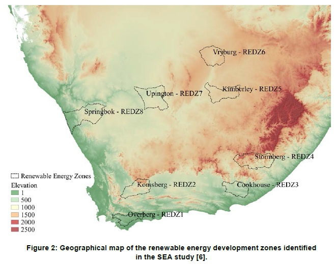
The SEA study conducted by CSIR identified eight geographical renewable energy areas to be targeted by future renewable energy projects. This study used criteria such as biodiversity, landscape, heritage areas, agriculture, socioeconomic considerations and the potential for renewable energy yield [5]. Identification of these zones allows environmental processes to be streamlined and fast-tracked and promotes the development of relevant infrastructure, such as electrical grid support.

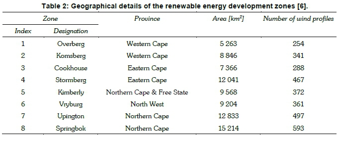
The REDZs are distributed over a considerable geographical area that represents diverse climatic conditions and seasonal characteristics. These areas include the Eastern Cape, Western Cape, North West, Free State and the Northern Cape, as shown in Figure 2. Table 2 summarises the geographical details of the various REDZs. The surface areas of the individual zones vary from 5 263 km² to 15 214 km², while the associated number of wind profiles varies from 254 to 593. It follows that there is considerable scope for the application of data reduction and classification methodologies with the view to assist in interpreting the properties of the wind resource comparatively for the individual zones.

 

3. Time-of-use tariff

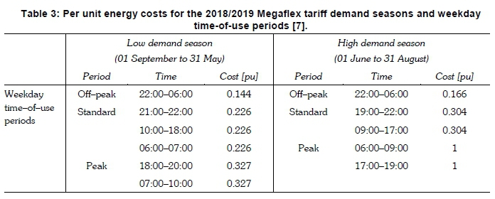
The Megaflex time-of-use (TOU) tariff system represents a useful reference for interpreting the diurnal and seasonal characteristics of renewable energy power generation profiles in the context of grid support. The tariff system gives a good indication of the running costs of the conventional generation fleet across diurnal and seasonal timelines [7]. Table 3 summarises the normalised per unit cost of energy for the 2018/2019 Megaflex TOU tariff for the annual demand seasons and the weekday diurnal TOU periods [7], using the peak period for the high demand season as reference. The energy cost for the weekday peak TOU periods in the high demand season exceeds the energy costs for the same TOU period in the low demand season by a factor of three. The energy costs for peak periods similarly exceeds the costs for standard and off-peak periods considerably. It follows that the grid impacts from the temporal renewable energy power generation profiles, including the impacts on energy balance and the overall cost of generation, are best interpreted in the context of the diurnal and seasonal temporal periods associated with the TOU tariff system.

 

4. Time series clustering methodologies

4.1 Overview

Clustering analysis typically involves the following well-defined steps [8]:

1. The sample set selected from the population database for clustering is chosen such that the population properties are reserved.

2. A similarity or dissimilarity measure is defined to determine a relationship between elements within a set. A similarity measure depicts a dependent relationship, where an increase in value correlates to an increase in likeness between two elements. A dissimilarity measure, in contrast, depicts an independent relationship, where an increase in value correlates to a decrease in likeness between two elements.

3. Based on the characteristics of the dataset to be clustered, a clustering algorithm is selected.

4. If necessary, the number of clusters is determined, as some clustering algorithms require a priori definition of this variable.

5. The clustering algorithm is implemented and the clustering outcomes are validated. The chosen clustering method must be capable of validation and replication within similar datasets.

4.2 Distance measures

The choice of the distance measure, defined as either a similarity or dissimilarity measure, is an important consideration in ensuring the accuracy of a clustering exercise. The distance measure is chosen by considering the characteristics of the dataset in conjunction with the clustering algorithm. Two of the most commonly used distance measures, namely the Euclidean distance and Pearson correlation distance, are considered in this investigation. The Euclidean distance, d_euc(x, y) is defined by the relationship [9]

where χ and y denote two vectors of length η within the dataset.

The Pearson correlation distance, d_cor(x,y), is defined by the relationship [9]

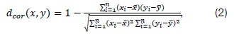
where χ and y denote the means of χ and y respectively. This correlation distance measures the linear relationship degree between elements χ and y.

4.3 Clustering algorithms

4.3.1 Partitioning algorithms

Partitioning methods involves the division of data into non-overlapping sub-sections. The process whereby the initial starting partitions are selected is a defining characteristic of this method. In some cases, these partitions are selected randomly, and other instances allow for user specification. Another defining characteristic involves the cluster type and the statistical criterion used for the assignment of data points or data vectors to the various clusters [10]. In some instances a point is assigned to the nearest centroid, while in other instances multiple passes are made and the centroids are updated repetitively. These methods require the number of clusters to be pre-selected, which forces outlier data to join one of the clustered solutions. The partitioning clustering algorithms considered in this study include k-means clustering, partitioning around me-doids (PAM) and the clustering large applications algorithm (CLARA).

The k-means algorithm requires a pre-defined number of clusters. Each cluster is represented by a centroid, which defines the homogeneous characteristics of that cluster. When computing the algorithm, data points are iteratively placed based on the similarity between an unassigned data point and the characteristics of the centroid within one of the clusters.

The un-clustered dataset, P, can be represented by the expression

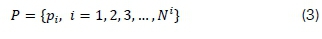
where p_; denotes the i^thelement and N^ldenotes the number of observations in the set. The set of clusters, C, can be represented by the expression

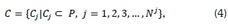
where Cj denotes the j^th cluster set and N-* denotes the number of clusters. The set of centroids associated with the clusters, W, is represented by the expression

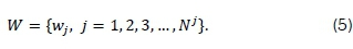
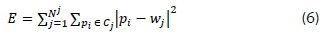
where wj denotes the j^th centroid. The k-means algorithm iteratively assigns each observation pi to a cluster Cj, based on the nearest centroid Wj. The centroid is also iteratively updated [11]. Once the data points have been assigned to a cluster, data points remain within their initially appointed clusters until convergence is reached. Convergence is reached when the error function, displays no significant change. The error function, E, commonly known as the total intra-cluster variation, is defined by the relationship [11]

The PAM algorithm, similar to the k-means algorithm, iteratively assigns the data vectors within a dataset to N^}pre-defined clusters. Each cluster is representative of the homogeneous characteristics displayed by the elements within the cluster, referred to as a cluster medoid. The medoid, when compared to all other members of its cluster, displays the smallest average dissimilarity [12]. This differs from k-means, as the centroid in k-means clustering is simply the mean value of the data vectors which constitute that specific cluster. The PAM method is, therefore, less susceptible to outliers and noise.

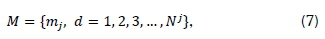
The CLARA algorithm is a k-medoids method, which is executed based on the PAM algorithm, except that it is adapted for much larger datasets. The algorithm begins by randomly sampling the full dataset and thereafter applying the PAM methodology to the sampled subsection [13]. A rating measure of suitability is calculated as the average sum of dissimilarities between data points contained in the full dataset and the closest medoid. The set of medoids, M, can be represented by the expression

where mj denotes the j^th medoid. The function expressing the rating measure, i?(rrij, P), is defined by the mathematical relationship [13]

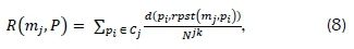
where rpst(m.j, p_t) represents the medoid which is closest to element p_t, d(pi, rpst(mj, p_t)) denotes the dissimilarity between a dataset element pi and rpst(rtij, Pi) and N^jkdenotes the number of elements in the j^th cluster. This process is then repeated and the sub-dataset with the smallest dissimilarity sum, using this measure, is retained.

Since all partitioning methods require an a priori definition of the number of clusters N^J, it is important to explore methods that can accurately and algorith-mically determine this value. Two methods for determining the number of clusters are explored, namely the elbow point method and silhouette analysis. The elbow point method calculates the total in-tra-cluster sum-of-squares as a function of the number of clusters. This function is then plotted and the elbow of the curve represents the optimal number of clusters, . Silhouette analysis determines the distance of separation between resulting clusters. This is typically expressed as a graphical display of the distance between each point within one cluster, to each point between the adjacent clusters. This metric lies in the range [-1, +1], where +1 represents a larger distance between points within adjacent clusters, 0 indicates a close or overlapping proximity and negative values indicate incorrect data point placements within a certain cluster. The silhouette width algorithm, similarly to the elbow method, is a function of N^j clusters. However, for each value of N^j, the average silhouette of the observation is calculated. The cluster number with the maximum average silhouette coefficient is then equal to the optimal number of clusters.

4.3.2Hierarchical algorithms

The hierarchical clustering algorithms considered in this study include agglomerative clustering and divisive analysis (DIANA) clustering. The agglomerative approach initialises with each element as a cluster, following which, clusters with the smallest sum-of-squared distance between them are merged with successive levelling. This iterative process continues until there is one large cluster representative of the entire dataset [8].

The divisive approach, inverse to the agglomer-ative approach, begins as a single cluster and successively divides the data into smaller clusters, based on the sum-of-squared distance. In both cases, a nested tree-like structure is created, which represents a hierarchy of partitions, where the number of partitions represents the number of elements within the dataset [14]. This creates non-overlapping clusters, with the notion that once assigned as member of a cluster, the body remains inseparable [15]. This treelike structure is called a dendrogram and, unlike in partitioning algorithms, this approach allows for the number of clusters to be determined after the algorithm is successfully completed. The entire hierarchy can be used as a single clustered solution, or various levels within the dendrogram can be selected as the optimal clustering solution.

4.3.3Fuzzy C-means algorithm

The fuzzy C-means clustering algorithm is an advanced methodology which allows dataset elements to belong to more than one cluster. It is based on the function [16]

where m denotes any real number, u_tj denotes the membership degree of an element pi within a cluster Cj and \\pi - Cj\\ the standard Euclidean distance between dataset elements pi and Cj to the clusters center. The function is subject to [16]

and

This process is repeated until [16]

Fuzzy C-means partitioning is an iterative process whereby cluster membership, as well as, the centroids of clusters are updated with each iteration.

4.4 Validation methods

A wide variety of clustering algorithms have been proposed in literature, each of which delivers a different level of competency depending on the characteristics of the dataset to which it is applied. Three commonly used internal validation methods are explored and applied in this study, namely the silhouette coefficient, the Calinski-Harabasz index and the Dunn index.

The silhouette coefficient for the i^thdataset element in a cluster, Sj, is defined by the relationship [16,18]

where a_tand b denote the mean intra-cluster distance and mean inter-cluster distance respectively, for every i^thelement. The mean nearest-cluster distance is defined by the relationship [18]

where B(i, k) represents the mean distance between the i^thelement and the elements in another cluster k. Equation 14 can also be expressed as [17]

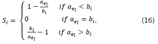
The coefficient Si lies within the range [-1, +1]. The value of the silhouette coefficient is closer to 1 if the element is assigned to the correct cluster. A negative value, however, indicates incorrect assignment of a dataset element.

The Calinski-Harabasz index, when maximised, indicates optimal clustering results. It is defined by the relationship [18]

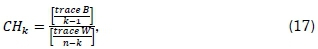
where k represents the number of clusters, ηthe total number of points within the dataset, Βthe error sum-of-squares between inter-clusters, and W the squared intra-cluster differences. The relationships for trace Βand trace W are defined by the equations [19]

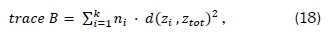
where n_; denotes the number of elements within cluster Cj and Zj is the center of cluster Cj; and

where χ denotes a dataset element which belongs to cluster Cj.

The Dunn index is defined by the mathematical relationship [20]

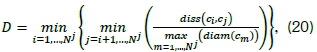
where N' denotes the number of clusters, diss(ci, Cj) represents the inter-cluster distance metric between clusters Cj and Cj, and diam(c_m) represents the intra-cluster diameter of cluster m. The inter-cluster distance is defined by the relationship

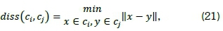
while the intra-cluster diameter is defined by

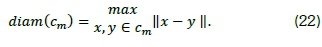
Larger Dunn index values indicate better cluster formations, i.e. well separated clusters with small cluster diameters. This suggests that maximising the inter-cluster distances, while minimising the intra-cluster distances, produces an optimal Dunn index result [21].

 

5. Case study results

5.1 Overview

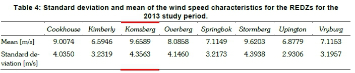
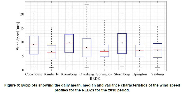
The case study is performed using a subset of the CSIR wind speed dataset, namely the temporal wind speed profiles for the 2013 calendar year. Table 4 presents the mean and standard deviation statistics of the wind speeds for the eight REDZs, for 2013. Figure 3 shows boxplots depicting the daily mean, median and variance characteristics. The results indicate that wind speed properties for the individual REDZs are quite diverse, with the mean wind speed varying from 6.5946 ms^-1 to 9.6589 ms^-1 and the standard deviation varies from 2.9306 ms^-1 to 4.3938 ms^-1. The Komsberg REDZ is selected for the detailed case study, as it displays high versatility; with the highest mean wind speed and a large standard deviation of the wind speed over the study period. In order to investigate the effects of seasonality, particularly in the context of the TOU tariff system, the input dataset is partitioned into the low demand and high demand seasons as defined by the Mega-Flex TOU tariff. Separate clustering exercises are then conducted for the chosen partitions.

5.2 Optimal number of clusters for partitioning algorithms

Two different methodologies, elbow point and silhouette width, are considered for determining the optimal number of clusters, k, for the partitioning clustering algorithms, i.e. k-means, PAM and CLARA. Since CLARA incorporates the PAM algorithm, the method for determining the optimal number of clusters is very similar to PAM, and this result is therefore omitted. The Euclidean distance measure is used for all of the clustering algorithms.

The elbow point method provides a visual illustration of the total intra-cluster sum-of-squares for various values of k. This allows the point to be identified at which an increase in the number of clusters shows limited further improvement. Figure 4 and Figure 5 show the total intra-cluster sum-of-squares obtained as a function of the number of clusters for the k-means algorithm and CLARA respectively. In both cases, the elbow point method suggests k = 4 as the optimal number of clusters. Although there is an improvement in the intra-cluster sum-of-squares from k = 4 to k = 5, it is not as significant as the change from k = 3 to k = 4.

 

 

 

 

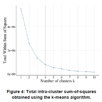
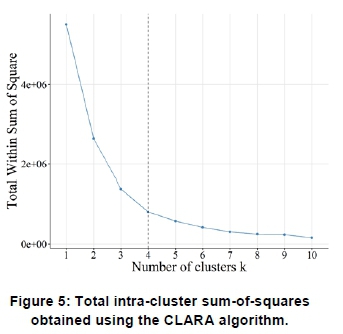
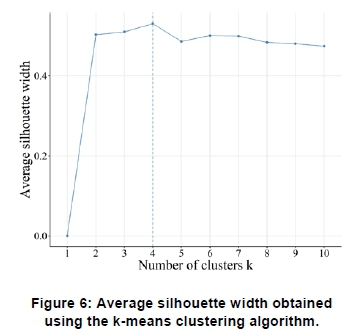
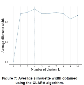
Figure 6 and Figure 7 shows the average silhouette width for k = 1 to k = 10. The highest coefficient value, or silhouette width, corresponds to the optimal k value. As in the case of the elbow point methodology, the silhouette width method depicts the optimal number of clusters at k = 4.

 

 

 

 

5.3 Clustering results

5.3.1 K-means clustering algorithm

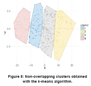
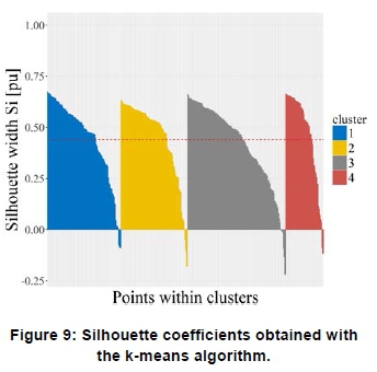
Figure 8 shows the non-overlapping clusters obtained with the k-means algorithm for the Komsberg wind speed profiles for the study period. Labels χ and y in Figure 8 denote the transformation of the initial variables within the dataset into a 2D representation of the set of variables through principal component analysis [22]. This dimensionality reduction algorithm creates a set of variables which can be seen as a projection or 'shadow' of the original dataset. Figure 9 shows the silhouette width of each cluster formed, which provides a visualisation of the validation metric. The degree of suitability of each data point to its assigned cluster is represented by the columns, where it can be seen that a fair number of profiles, i.e. 14, yield negative silhouette widths. This indicates that these negative cluster assignments have a low degree of similarity to the characterising function of the cluster and are most likely better suited in a different cluster. Visualisation of the silhouette widths for each dataset point assignments gives a good indication of the accuracy of the implemented clustering algorithm.

 

 

 

 

5.3.2 Partitioning around medoids clustering algorithm

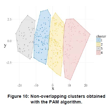
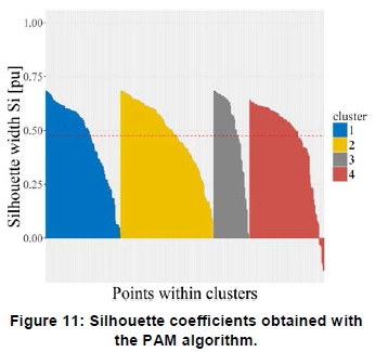
Figure 10 shows the non-overlapping clusters obtained with the PAM algorithm for the Komsberg wind speed profiles for the study period. The cluster structures are very similar to the structures obtained with the k-means clustering algorithm. Figure 11 shows that a relatively low number of profiles, i.e. 6, yield negative silhouette widths. This algorithm, however, shows a better assignment of the profiles compared to the k-means algorithm.

 

 

 

 

5.3.3Clustering large applications algorithm

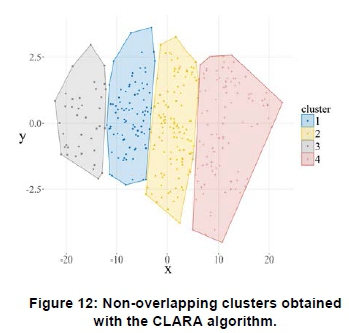
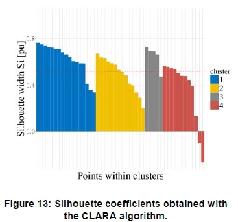
Figure 12 shows the non-overlapping clusters obtained with the CLARA algorithm for the Komsberg wind speed profiles for the study period. The CLARA method selects a sub-dataset of the original dataset and partitions this sub-dataset into k clusters using the PAM algorithm. Once a representative object has been defined for each of the k clusters within the sub-dataset, namely the cluster medoid, the remaining observations within the entire dataset are assigned to the nearest medoid. Figure 13 shows the initially clustered sub-dataset using the CLARA method, which depicts a low number of profiles, i.e. 2, yield negative silhouette widths. The result shows a better assignment of the profiles compared with both the k-means and PAM algorithms.

 

 

 

 

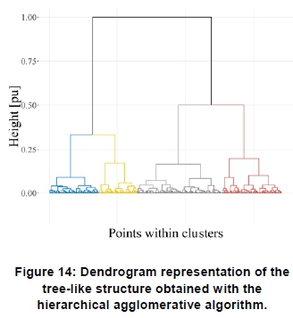
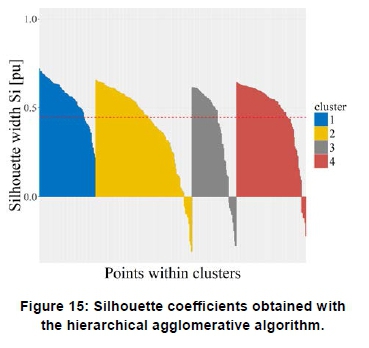
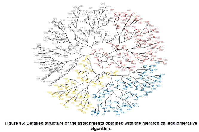
5.3.4Hierarchical agglomerative algorithm

Figure 14 shows a dendrogram of the cluster assignments obtained using the hierarchical agglomerative algorithm. The dendrogram depicts a tree-like structure representation of the cluster assignments. Figure 15 shows that a relatively high number of profiles, i.e. 26, yield negative silhouette widths. Figure 16 shows an alternative, more detailed, structural representation of the cluster assignments obtained with the algorithm.

 

 

 

 

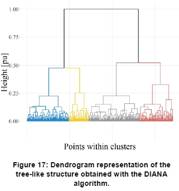
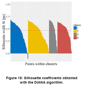
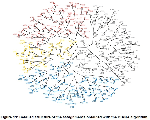
5.3.5 Divisive analysis algorithm

Figure 17 shows a dendrogram of the cluster assignments obtained using the DIANA algorithm. Figure 18 shows that a relatively low number of profiles, i.e. 4, yield negative Silhouette widths. This shows a better cluster assignment compared to the hierarchical agglomerative algorithm. Figure 19 shows an alternative, more detailed, structural representation of the cluster assignments obtained with the algorithm.

 

 

 

 

5.3.6 Fuzzy C-means clustering

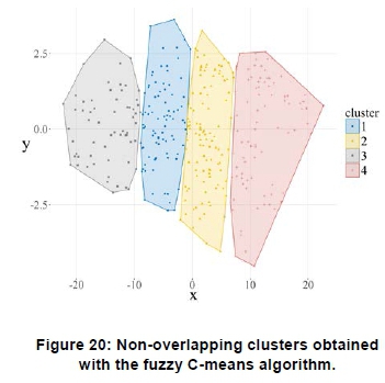
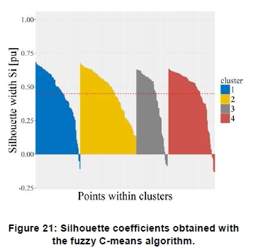
Figure 20 shows the non-overlapping clusters obtained with the fuzzy C-means algorithm. Figure 21 shows that a fair number of profiles, i.e. 16, yield negative silhouette widths. This method shows a high number of incorrectly assigned clusters despite being a higher level clustering algorithm.

 

 

 

 

5.4 Comparison of validation metrics

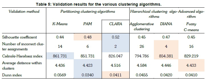
Table 5 summarises the results of the validation methods applied for the various clustering algorithms, i.e. the Silhouette coefficient, Calinski-Harabasz index and Dunn index. Table 5 also gives two other complementary values of interest, namely the number of incorrect cluster placements and the average distance within clusters. The blue and orange shaded results in Table 5 indicate the best and second-best validation results respectively. Overall, the PAM algorithm and the CLARA algorithm yield optimal validation results. The CLARA sampling model uses a reduced representation of large datasets, which decreases the algorithmic computing time while retaining an accurate dataset representation. This algorithm also yields the highest Silhouette coefficient, with an average intra-cluster distance output only fractionally behind the PAM algorithm. Since this algorithm can be easily applied to larger datasets, it is concluded that CLARA method represents the best performing algorithm for this application.

5.5 Detailed results obtained using CLARA

The CLARA algorithm is applied to both the high demand and the low demand season wind speed profiles for 2013 in the Komsberg REDZ. This allows for the comparison of the wind resources found in this zone, in the context of TOU demand seasons.

5.5.1 High demand season clustering results

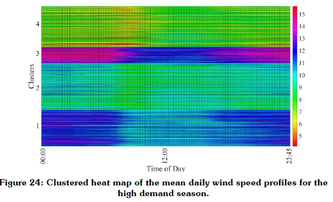
Figure 22 shows the mean daily wind speed profiles for the high demand season, where the different colours indicate the different clusters. The colour assignments are the same as shown in Figure 13: Silhouette coefficients obtained with the CLARA algorithm. Figure 24 depicts the same information shown in Figure 22, but in the form of a heat map. These representations allow for interpretation of the mean yield of the various clusters in the context of daily TOU periods. The results show that cluster 3 exhibits the highest average daily wind speed, i.e. of the order of 13.3 m/s. Cluster 3 also exhibits high average wind speeds from 16:00 until 10:30. This is a good trait for grid support, as the two peak TOU periods occur from 06:00 to 09:00 and from 17:00 to 19:00 respectively. This cluster, furthermore, exhibits good compatibility with solar PV generation, as it supports the cumulative renewable energy generation profile outside the daily solar generation cycle.

 

 

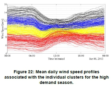
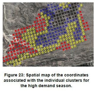
Figure 23 shows a geographical map of the clusters. As expected, the cluster assignments are closely related to the underlying topographical features of the profile coordinates. The spatial distributions represent well-defined spatial clustered areas.

 

 

5.5.2 Low demand season clustering results

Figure 25 shows the non-overlapping clusters obtained with the CLARA algorithm for the low demand season. Figure 26 shows the initial clustered sub-dataset using the CLARA method, which depicts a low number of profiles, i.e. 2, yield negative silhouette widths.

 

 

 

 

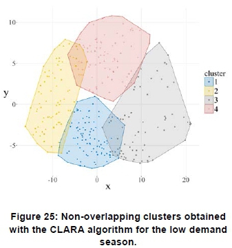
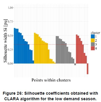
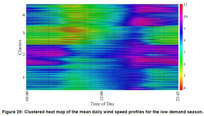
Figure 27 shows the mean daily wind speed profiles for the low demand season, where the different colours indicate the different clusters. The colour assignments are the same as shown in Figure 26. Figure 29 depicts the same information shown in Figure 27, but in the form of a heat map. Cluster 2 exhibits the highest average daily wind speed, i.e. of the order of 8.8 m/s. Cluster 2 and cluster 4 exhibit high average wind speeds from 18:00 until 00:00. This is a good trait for grid support as one of the peak TOU periods occur between 17:00 and 19:00.

 

 

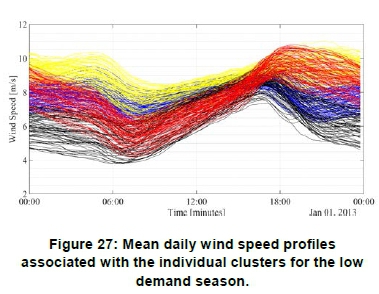
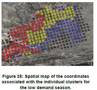
Figure 28 shows a geographical map of the clusters. As in the case of the high demand season, the clusters represent well-defined spatial areas. The geographical assignments differ to from the assignments shown in Figure 23. This emphasises the importance of clustering based on the power producers' main energy yield goal.

 

 

5.5.3 Comparison between the high and low demand season clustering results

The results presented in Figure 22 and Figure 27 shows that the spread of the individual mean daily profiles is significantly smaller for the low demand season than the high demand season. This may be related to the increased number of days associated with the averaging process for the low demand season, which indicates the potential need for further temporal partitioning of the low demand season dataset.

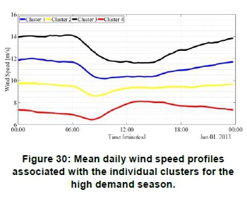
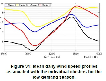
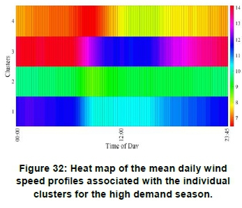
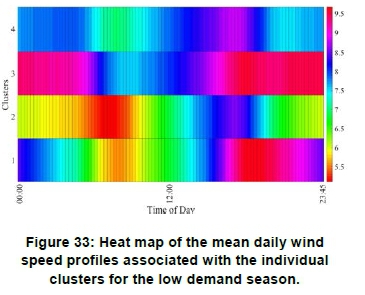
Figures 30 and 31 show the mean daily profiles of the clusters obtained for the high demand and low demand seasons repectively. Figures 32 and 33 depict the same information in the form of heat maps. The mean daily profiles associated with the individual clusters for a given demand season differ substantially, both with reference to the mean daily wind speeds, as well as, the temporal diurnal cycles. This observation also applies when comparing the clustered mean daily profiles obtained for the different demand seasons. In general, the low demand season exhibits lower mean daily wind speeds compared to the high demand season. This is an indication that the seasonal wind energy yield in the Koms-berg REDZ correlates well with the seasonal national demand, which is embodied in the Megaflex TOU tariff.

The results presented in Figures 30 to 33, when viewed in combination with the spatial maps shown in Figure 23 and Figure 28, are potentially very useful for high level planning studies aimed at optimising the renewable energy plant siting, based on wind generation capacity for optimum grid support, especially in the context of reducing the variability of the residual load profile. The clustered wind profiles shown in Figure 30, for the high demand season, exhibit reduced yield at midday for clusters 1 and 3. These clusters are therefore suitable for combined wind and solar applications in the context of reducing variability of the aggregated mean daily profile. Cluster 3, however, exhibits a more even daily wind speed profile, while cluster 4 shows an increase in midday energy production. The profiles shown in Figure 31, for the low demand season, show contrasting results, where a dip in wind speed occurs in the early morning around 6:00, with a strong peak around 18:00.

 

 

 

 

 

 

 

 

 

6. Conclusion

This study investigated the performance of various clustering algorithms, namely k-means, partitioning around medoids, clustering large applications algorithm, agglomerative clustering, divisive analysis and fuzzy C-means, for clustering the temporal wind speed profiles associated with specific geographical areas. Two distance measures, namely the Euclidean distance and Pearson correlation distance, were considered. The validation metrics evaluated in the investigation include the silhouette coefficient, Calinski-Harabasz index and the Dunn index. The algorithmic comparison tests are performed for the Komsberg renewable energy development zone (REDZ), using the spatio-temporal, meso-scale renewable energy resource dataset produced for Southern Africa by the Council of Scientific and Industrial Research. The Komsberg REDZ is selected since this zone displays high wind speed variability and topographical range.

The results show that the CLARA algorithm, paired with the Euclidean distance metric, produces the best clustering results. The clustering exercise yields an optimum of four clusters for the Komsberg zone, which represents a good data reduction result for high level interpretation of the wind resource properties of the underlying spatial coordinates. The clusters are well defined from the perspectives of the associated mean daily temporal wind speed profiles and the spatial distributions. It is shown that the temporal properties of the mean daily wind speed profiles associated with the individual clusters are quite diverse and, furthermore, differ markedly for the high demand and low demand seasons defined by the Megaflex TOU tariff. In the context of grid support, this study is important in identifying optimal siting areas for wind energy facilities in the zone.

Clustered temporal wind speed profiles represent a valuable resource for understanding and interpreting the characteristics of the wind resource associated with a geographical area for medium- and longterm siting studies aimed at maximising grid support. Clustered wind resource maps should, ideally, be developed for the entire wind resource dataset. The clustered wind speed profiles, furthermore, represent a highly reduced dataset that is useful for computationally intense data manipulation exercises involving machine learning, optimised renewable energy capacity allocation and siting, and the development of forecasting models.

 

Acknowledgements

The authors gratefully acknowledge the support of the Doug Banks Renewable Energy Vision, CSIR and Eskom Tertiary Education Support Program in conducting this research.

Author roles

Chantelle Janse van Vuuren: analytical techniques, data collection, simulation running and write-up. Hendrik J Vermeulen: Research suggestions and formulation, write-up editing.

 

References

[1] L. Hirth, The market value of variable renewables: The effect of solar wind power variability on their relative price, Energy Economics, vol. 38, pp. 218-236, 2013.         [ Links ]

[2] Council for Scientific and Industrial Research, National wind solar sea, Council for Scientific and Industrial Research, [Online]. Available: https://www.csir.co.za/national-wind-solar-sea. [Accessed 08 10 2018].         [ Links ]

[3] J. Michalakes, J. Dudhia, D. Gill, T. Henderson, J. Klemp, W. Skamarock and W. Wang, The weather reseach and forecast model: Software architecture and performance, in Use of high performance computing in meteorology, World Scientific Publishing Co Pte Ltd, 2018.         [ Links ]

[4] Fraunhofer IWES and The CSIR Energy Centre, Wind and solar PV resource aggregation study for South Africa, Fraunhofer IWES, South Africa, 2016.         [ Links ]

[5] Council for Scientific and Industrial Research, Strategic search for SA's best wind and sun, Council for Scientific and Industrial Research, 2014.         [ Links ]

[6] C. Y. Janse van Vuuren, H. J. Vermeulen and J. C. Bekker, Clustering of wind resource Weibull characteristics on the South African renewable energy development zones, in The 10th International Renewable Energy Congress (IREC 2019), Sousse, Tunisia, 2019.         [ Links ]

[7] Eskom, tariffs & charges 018/2019, Eskom, 2018.         [ Links ]

[8] C. Martha, W. Milligan and G. Cooper, Methodology review: Clustering methods, Applied Ssychological Measurement, vol. 11, no. No.4, pp. 329-354, 1987.         [ Links ]

[9] A. Kassambara, Clustering distance measures, in Practical guide to cluster analysis in R, STHDA, 2017, pp. 25-27.         [ Links ]

[10] S. Ayramo and T. Karkkainen, Introduction to partitioning-based clustering methods with a robust example, University of Jyvaskyla Department of Mathematical Information Technology, Jyvaskyla, 2006.         [ Links ]

[11] K. Alsabti, S. Ranka and V. Singh, An efficient k-means clustering algorithm, in Electrical Engineering and Computer Science, 1997.         [ Links ]

[12] M. A. Mottalib and F. B. A. Abid, An accurate grid-based PAM clustering method for large dataset, International Journal of Computer Applications (0975 - 8887), vol. Volume 41, no. No.21, p. 0975 - 8887,2012.         [ Links ]

[13] A. Bhat, k-medoids clustering using partitioning around medoids for performing face recognition, International Journal of Soft Computing, Mathematics and Control, vol. Vol. 3, no. No.3, 2014.         [ Links ]

[14] D. S. Wilks, Chapter 15 - Cluster analysis, in International geophysics, Elsevier, 2011.         [ Links ]

[15] G. Milligan, An examination of the effect of six types of error perturbation on fifteen clustering algorithms, Psychometrika, vol. 45, no. 3, pp. 325-342, 1980.         [ Links ]

[16] J. Keane, A. Stetco and . X.-J. Zeng, Fuzzy C-means+ + : Fuzzy C-means with effective seeding initialization, Expert Systems with Applications, vol. 42, p. 7541-7548, 2015.         [ Links ]

[17] Suranaree University of Technology, The clustering validity with silhouette and sum-of-squared errors, in Industrial Application Engineering, Japan, 2015.         [ Links ]

[18] B. Kim, J. Kim and G. Yi, Analysis of clustering evaluation considering features of item response data using data mining technique for setting cut-off scores, Symmetry MDIP, p. 8, 25 April 2017.         [ Links ]

[19] S. Saitta, B. Raphael and I. F. C. Smith, A comprehensive validity index for clustering, Intelligent Data Analysis, vol. 12, no. 6, pp. 529-548, November 2008.         [ Links ]

[20] F. Kovács, C. Legány and A. Babos, Cluster validity measurement techniques, Department of Automation and Applied Informatics,Budapest University of Technology and Economics, Budapest, Hungary.         [ Links ]

[21] S. Saitta, B. Raphael and I. F. Smith, A bounded index for cluster validity, in Ecole Polytechnique Fédérale de Lausanne, Switzerland.         [ Links ]

[22] I. Jolliffe, Principal component analysis, in International Encyclopedia of Statistical Science, Berlin, Heidelberg, Springer, 2011.         [ Links ]

[23] University of Reading, Wind profile program-Logarithmic wind profile, [Online]. Available: http://www.met.reading.ac.uk/~marc/i^wind/interp/log_prof/. [Accessed 2018 July 19].         [ Links ]

[24] A. Kassambara, K-means clustering, in Practical guide to cluster analysis in R, STHDA, 2017, pp. 36-38.         [ Links ]

[25] A. Kassambara, K-Medoids, in Practical guide to cluster analysis in R, STHDA, 2017, pp. 36-37.         [ Links ]

[26] A. Kassambara, Internal measures for cluster validation, in Practical guide to cluster analysis in R, STHDA, 2017, pp. 139-140.         [ Links ]

[27] S. Aranganayagi and K. Thangavel, Clustering categorical data using silhouette coefficient as a relocating measure, in International Conference on Computational Intelligence and Multimedia Applications, Sivakasi, Tamil Nadu, India, 2007.         [ Links ]

[28] F. Hoppner, F. Klawonn, R. Kruee and T. Runkler, Fuzzy cluster analysis, New York: John Wiley & Sons, LTD, 2000.         [ Links ]

[29] A. Kassambara, CLARA - Clustering large applications, in Practical guide to cluster analysis in R, STHDA, 2017, pp. 57-63.         [ Links ]

[30] M. B. Eisen, P. T. Spellman and P. O. Brown, Cluster analysis and display of genome-wide expression patterns, Proceedings of the National Academy of Sciences, p. 14863 - 14868, 08 November 1999.         [ Links ]

[31] R. Tibshirani, G. Walther and T. Hastie, Estimating the number if clusters in a data set via the gap statistic, Royal Statistical Society, USA, 2001.         [ Links ]

[32] A. Trevino, Introduction to K-means clustering, 06 December 2016. [Online]. Available: https://www.datascience.com/blog/k-means-clustering. [Accessed 07 October 2018].         [ Links ]

[33] R. Lletia, M. OrtizaL, A. Sarabiab and M. Sánchezb, Selecting variables for k-means cluster analysis by using a genetic algorithm that optimises the silhouettes, Analytica Chimica Acta, vol. 515, no. 1, pp. 87-100, 2003.         [ Links ]

 

 

* Corresponding author: Tel:+27 (0)76 070 4573; email: jansevanvuurenchantelle@gmail.com