ARTICLES

 

Cluster analysis for classification and forecasting of solar irradiance in Durban, South Africa

 

 

Paulene Govender^{I, *}; Michael J. Brooks^II; Alan P. Matthews^I

^ISchool of Chemistry and Physics, University of KwaZulu-Natal, P. Bag X54001, Durban 4000, South Africa
^IISchool of Engineering, University of KwaZulu-Natal, P. Bag X54001, Durban, 4000, South Africa

 

 

---

ABSTRACT

Clustering of solar irradiance patterns was used in conjunction with cloud cover forecasts from Numerical Weather Predictions for day-ahead forecasting of irradiance. Beam irradiance as a function of time during daylight was recorded over a one-year period in Durban, to which k-means clustering was applied to produce four classes of day with diurnal patterns characterised as sunny all day, cloudy all day, sunny morning-cloudy afternoon, and cloudy morning-sunny afternoon. Two forecasting methods were investigated. The first used k-means clustering on predicted daily cloud cover profiles. The second used a rule whereby predicted cloud cover profiles were classified according to whether their average in the morning and afternoon were above or below 50%. In both methods, four classes were found, which had diurnal patterns associated with the irradiance classes that were used to forecast the irradiance class for the day ahead. The two methods had a comparable success rate of about 65%; the cloud cover clustering method was better for sunny and cloudy days; and the 50% rule was better for mixed cloud conditions.
Highlights:
• Clustering produced four classes of beam irradi-ance profiles for Durban
• Numerical weather prediction cloud cover patterns into four classes
• Association of classes used for day-ahead forecasting of beam irradiance
• Forecasting had a moderate success rate of about 65%

Keywords: numerical weather prediction; cloud cover; k-means; classes

---

 

 

Nomenclature

Abbreviations

NWP numerical weather prediction

SUI solar utility index

GHI global horizontal irradiance

DHI diffuse horizontal irradiance

DNI direct normal irradiance

NOAA National Oceanic and Atmospheric Administration

ANN artificial neural network

TOA top of atmosphere

SAST South African standard time

PCA principal component analysis

RMSE root mean square error

Symbols

k_t clearness index

k_b direct horizontal irradiance fraction

B beam irradiance

B_n normalised beam irradiance

B_c Ineichen model clear sky beam component

hourly average of the normalised beam irradiance

n number of minutes

i minute index

T_L Linke turbidity coefficient

C cloud cover percentage

SI silhouette index

average silhouette index for an individual cluster

average silhouette index for the entire set of objects in a cluster

Cam morning cloud cover average

C_PM afternoon cloud cover average

 

 

1. Introduction

Characterisation and forecasting of solar irradiation patterns has become increasingly important for designing, operating and managing grid-connected solar power plants. Knowledge of typical solar irradi-ance at a given location, and how it varies from day to day, allows power plant operators to estimate power output. It is also useful for forecasting power output because knowledge of common irradiance patterns may be used to constrain a forecast to fall with a high probability into one of those patterns.

An approach to understand solar resource patterns includes classification and characterisation of irradiance profiles by cluster analysis, where a profile is defined as irradiance and a function of time over a day. Classification is useful for forecasting because, if the class of a day can be successfully forecast, the irradiance profile of that day would share the general pattern of the class. Forecasting employs a range of techniques, including using NWP and satellite imagery of cloud cover to predict how cloud cover changes over space and time (Inman et al., 2013). Several studies (Mathiesen et al., 2013; Lorenz et al., 2009; Remund et al., 2008; Perez et al., 2007; Aguiar et al., 2016) successfully employed NWP models together with other techniques for solar forecasts.

Other studies (Muselli et al., 2000; Maafi and Harrouni, 2003; Diabaté et al., 2004; Harro uni et al., 2005; Soubdhan et al., 2009; Gaste)n-Romeo et al., 2011 and Zhandire, 2017) investigated classification of days based on solar irradiance but did not consider forecasting. The irradiance characteristics of Durban, KwaZulu-Natal Province, South Africa, which has a humid sub-tropical climate and significant cloud variation, has been described by Lysko (2006), Zawilska and Brooks (2011) and Kunene et al. (2013), but not using clustering of irradiance profiles. Clustering was used by Zhandire (2017) to produce classes of a SUI for each of nine stations across South Africa. The SUI was a daily average of beam and diffuse horizontal irradiance. Zhandire did not consider beam irradiance independently or the diurnal variation of beam irradiance. In addition, the primary aim of that study was to provide a new solar resource index for classification for multiple stations across South Africa, and did not aim exclusively to characterise the solar irradiance patterns in Durban or investigate the possibility of forecasting using classification results.

The most commonly-used classification variable is k_t, which is the ratio of the measured GHI to the TOA irradiance. Studies that use classification for forecasting include those by McCandless et al. (2014, 2015), where identification of different cloud regimes, subsequently solar irradiance forecasting models: ANNs, were built specifically to predict kt for each regime. McCandless et al. (2014) tested forecasts up to three hours ahead, and McCandless et al. (2015) used k-means clustering to identify seven cloud regimes based on the previous 45 minutes of k_tfor a 15-minute forecast. McCandless et al. (2014) identified cloud regimes by k-means clustering but tested forecasts up to three hours ahead rather than day forecasts. Furthermore, McCandless et al. (2015) merely considered the use of NWPs for forecasting without applying it.

Badosa et al. (2013) presented a characterisation of mesoscale and local-scale solar irradiance variability for Reunion Island, which showed that the island's diurnal irradiance variation can be classified into five classes. Badosa et al. (2015) explored the variability in local irradiance conditions and cloud cover dynamics of Reunion Island using irradiance classes defined in Badosa et al. (2013) together with synoptic wind and relative humidity parameters. Jeanty et al. (2013) investigated irradiance patterns for Reunion Island using cluster analysis applied to daily profiles of direct horizontal irradiance fraction, kb, defined as 1 - DHI/GHI, where DHI is diffuse horizontal irradiance. Similar to Badosa et al. (2013), the study revealed five dominant patterns for the island. However, only four of the five patterns, corresponding to clear, cloudy, AM clear and PM clear conditions, are positively correlated with the classes obtained by Badosa et al. (2013).

Badosa et al. (2013; 2015) and Jeanty et al. (2013) served as a basis for much of the present study, where minute-resolution irradiance profiles similar to those of Jeanty et al. were pre-processed by PCA and then clustered by the k-means method. This method produced a set of classes of differing diurnal variation that characterise the irradiance patterns in Durban. Clustering was also applied to hourly-averaged beam irradiance, and the classes obtained were compared with those obtained from the minute-resolution data. Although knowledge of both beam and global irradiance is important for solar power plants, the present investigation was restricted to beam irradiance to test a method suitable for extension to forecasting of global irradiance. Presented here is an approach that applies clustering to both radiometric data and NWP cloud cover for day-ahead forecasting of direct (beam) irradiance, which is tested against a simple decision rule using morning and afternoon averages of cloud cover. The NWP provides day-ahead cloud cover forecasts with an hourly temporal resolution, and cloud cover is used here for forecasting because of its strong association with beam irradiance intensity.

The forecasting model starts with an NWP day-ahead forecast of hourly cloud cover percentage and uses it to predict the irradiance class for that day. This is compared with the day's actual irradiance class, and the predicted irradiance profile is the mean profile of the class, which is compared with the actual irradiance profile of the day. In Section 2, the radiometric data used for this study is described and the variables used for clustering and forecasting are defined. The section also includes a motivation for the choice of the beam irradiance component for clustering and forecasting. Thereafter details of the clustering and forecasting methods are described. In Section 3, results of the clustering of radiometric and cloud cover data are given. Forecasting results are also presented, including a comparison of the performance of the two forecasting methods. A discussion of the clustering and forecasting results is presented in Section 4. Conclusions of the main findings are given in Section 5.

 

2. Method

2.1 Data and definition of variables

Irradiance data were collected at the University of KwaZulu-Natal, Durban, South Africa (29.87° S; 30.98° E). The radiometric station, which is part of the SAURAN network (Brooks et al., 2015), is located 150 m above mean sea level, on a roof platform. Measurements for DNI were obtained using a Kipp & Zonen CHP1 pyrheliometer. The instrument was mounted on a Solys2 automatic sun tracker. Measurements were taken every two seconds and averaged over one-minute intervals. Daily profiles of DNI were recorded at one-minute intervals from 8:30 to 16:30 solar time. This restricted time interval was chosen to avoid sensor shading during early morning and late afternoon in winter. The radio-metric data were manually checked for quality and to identify anomalies. This was coupled with a forecast of hourly C obtained from AccuWeather, a public weather service provider, to produce a daily profile from 9:00 to 16:00 SAST. The output was derived from an NWP model run by the NOAA.

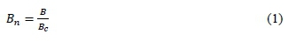
The irradiance measurements were used to define minute-resolution and hourly-resolution profiles for clustering. Let B denote beam irradiance (DNI) at one-minute resolution, where B_nn is defined as B normalised to the beam component Bc_nn of the Ineichen clear sky model (Ineichen and Perez, 2002) for Durban as expressed by Equation 1.

Then, let denote the hourly average of B_n to produce Equation 2.

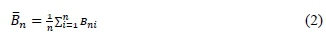
where i is the minute index and n = 60. The first minute (i = 1) is on the half-hour, e.g. 9:30, values of B_nare known at times 9:00, 10:00, 11:00,... 16:00.,

The normalised beam irradiance, B„_;, is used rather than beam fraction k_b, because it removes seasonality. Near dawn and dusk, DNI is close to zero, and DHI is almost equal to GHI, therefore, k_b«0. On a clear day, k_b rises in the first hour after dawn to near unity and declines in late afternoon during the last hour before sunset. As the seasons change, sunrise and sunset times change, causing the k_b profiles to vary in the start and end times of the rising and declining phases. This seasonal variation in profile, even for clear days, creates differences that are not produced by cloud conditions. Given that a primary objective was to cluster profiles in accordance with how they are affected by clouds, B_n was chosen rather than k_b because the shape of the B_n profile is independent of seasonality. The Bn is zero before sunrise and after sunset and these times vary with season; and between these times its shape depends on cloud conditions, but for a clear day, its profile is a horizontal line. Figure 1 shows k_b for B_c, the clear-sky beam, for the winter and summer solstices, where k_b= 1 - DJG_c, and the Ineichen clear sky model diffuse and global irradiance are D_cand G_c, respectively.

 

 

The Ineichen model is preferred over other clear sky models since the only atmospheric parameter required is the Linke turbidity coefficient T_Lfor the location. Monthly averages of the T_L values for Durban were estimated using local radiometric data with the MATLAB implementation of the clear sky model developed by Sandia National Laboratories (SNL, 2012).

2.2 Clustering

For data with high dimensionality, in this case B_n, PCA was performed prior to clustering as a pre-processing step. The method was implemented in MATLAB (R2015a) using the Statistics Toolbox. The PCA reduces the dimensionality of a data set, while preserving most of the variance in the data. As described by Jolliffe (2002), this is achieved by transforming to a new set of axes, called principal components, which are ordered successively so that the first few components retain most of the variation present in the original data. The cumulative percentage of the total variation was used to choose the minimum number of principal components to be retained, where the minimum number of components with a cumulative percentage of 90% was retained.

To obtain classes of pre-processed Bn, and of and C, k-means clustering was applied, also implemented in MATLAB. The k-means algorithm, developed by MacQueen (1967) is a well-known and commonly-used partitional clustering algorithm (Halkidi, 2001). It partitions a set of n objects into k clusters, where the number of clusters, k, is specified in advance. In this case, each object is a daily profile of one of the variables defined above. The profile may be represented by a position in a multi-dimensional space on which a metric is defined to calculate the distance between positions. According to Rous-seeuw (1957), the compactness and separation of clusters is quantified by the SI, which varies from -1 to 1, where an SI that approaches 1 is indicative of an object being 'well-clustered'. On the other hand, SI approaching -1 indicates that the object is not well-suited to that cluster (Zagouras et al., 2014; Rousseeuw, 1957). The average SI for an individual SI_C, where C is a cluster label, or for the entire set of objects (denoted here as ) is used as an index of overall clustering compactness. Lleti et al. (2004) consider a silhouette value of 0.6 or greater to be a good clustering result, which will be used here as a criterion for acceptable compactness. The number of clusters was not determined by a specific criterion, but by consideration of the results for various values of k, guided by well as values of SI_Cfor each cluster. The aim of the present study was to find the 'natural' clustering, which corresponds with finding the largest number k of compact clusters. The guideline used was to maximise k, while keeping greater than 0.6 and seeking to maintain as high as possible for each of the clusters obtained. Classification of daily profiles was based on the clusters that were determined, the terms 'cluster' and 'class' are used interchangeably.

2.3 Forecasting

Let the class mean profile (B_n) denote the mean of the set of B_nprofiles for a class. Forecasting was done by using a day-ahead forecast of C to forecast the class of the day and then using (B_n) for that class as the forecast of the B_nprofile. Although C was specified on the hour in 'clock time' (SAST), and hence offset from solar time, the difference of at most 20 minutes was small compared with the one-hour resolution of the C profile and was not significant. Forecasting was done using two methods. The first uses classes of C found by k-means clustering. The forecast of C is assigned to one of the classes, which in turn is associated with one of the classes of B_n. The second method, the '50% rule', uses a set of decision rules based on C. Both methods depend on the clustering results and these are described further in Section 3. The profiles forecast using both methods are compared with the actual B_nfor the day by computing the RMSE given by Equation 3.

where and are the actual and forecast profiles, respectively, and n is the number of hours in the time interval. The actual profile is that derived from radiometric measurements, whereas the forecast profile is the mean profile of the class that is forecast.

 

3. Results

3.1 Data

For clustering of radiometric data to establish classes, the set contained 365 days from 28 January 2014 to 27 January 2015. Clustering of cloud cover (from NWP forecasts) was applied to a set of 243 days in 2016, approximately uniformly distributed throughout the year, where missing days were almost all weekends. There was no requirement that the radiometric data and NWP cloud cover be in the same year because clustering was applied to find patterns that were independent of a specific year. Testing of forecasting was done using a set of 100 days in 2017, including most days during the months of January to June.

3.2 Clustering of minute-resolution normalised beam irradiance

Each daily profile of B_nconsisted of a set of 481 values for each minute during the interval 8:30 to 16:30 solar time. Therefore, each Bn profile corresponded to a point in a 481-d space, which was reduced to a low-dimensional space by PCA. The first eight components accounted for 90% of the variance and were hence retained.

The clustering results for the daily profiles of Bn in 8-d space were almost identical to those for B_n, producing identical classes with identical members, consequently only the results of clustering of B_nare presented. This high degree of similarity indicates that the sub-hourly temporal structure in Bn did not result in any significant difference in clustering compared with the temporal structure in the hourly average.

3.3 Clustering of hourly-resolution normalised beam irradiance

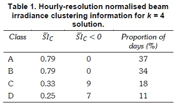
The daily profiles of were clustered using k-means for k = 4, since = 0.65 was found to be the highest for 4 clusters. This was selected as the final clustering result. Clusters A and B have SI_C of 0.79, and clusters C and D have SI₃ = 0.33 and SI₄ = 0.25. Table 1 summarises the clustering information.

 

 

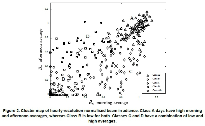
The four clusters are represented in Figure 2, which shows morning (8:30-12:30) average of on the horizontal axis and afternoon (12:30-16:30) average on the vertical axis. Clusters A and B are compact and widely separated, whereas clusters C and D, in the region between A and B, are less compact and have members at their edges that are closer on average to A and B than to their own cluster, resulting in negative SI for those members. A minor difference between the B_nand Bn clustering is that the number of profiles with negative SI decreased from 19 for Bn to 16 for B_n.

Since beam irradiance is strongly correlated with cloud cover, Figure 3 shows that there are four classes of diurnal variation in beam irradiance on the half-day scale: sunny all day (cluster A); cloudy all day (cluster B); sunny in the morning and cloudy in the afternoon (cluster C); and cloudy in the morning and sunny in the afternoon (cluster D). These clusters are hence identified as irradiance pattern classes, which are labelled as: Class A: sunny, Class B: cloudy, Class C: sunny AM-cloudy PM, and Class D: cloudy AM-sunny PM. The diurnal patterns shown in Figure 2 are evident in the class mean profiles plotted in Figure 3.

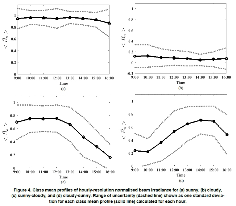
It is important to have knowledge of the range of uncertainty for forecasting, which is shown in Figure 4(a)-(d) as plots of standard deviation for each class mean profile, calculated for each hour. The more compact clusters, A and B, have lower standard deviation than the less compact clusters, C and D. A forecast that places a day into a class will, therefore, be predicted to have an irradiance profile similar to that class mean profile within an uncertainty corresponding to the class standard deviation. It is, therefore, expected that forecasts of A and B class will have less uncertainty than for C and D.

3.4 Clustering of cloud cover

It was necessary to have four classes of cloud cover in order to use classes of C to forecast the irradiance class. Because low B_nis correlated with high C, it was expected that they should exhibit similar clustering, considering that NWP is designed to model the weather pattern as accurately as possible. It was found that k = 4 was a good solution, with SI_TOT = 0.74. Table 2 summarises the results of clustering of daily C profiles.

 

 

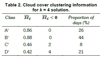
Figure 5 shows a cluster map with morning average of C on the horizontal axis and the afternoon average on the vertical axis. The four clusters have cloud cover conditions that are associated with the B_nclasses and are given the same labels, but with primes. The C classes are, therefore, Class A': low C all day, Class B': high C all day, Class C': low C in the morning and high C in the afternoon, and Class D': high C in the morning and low C in the afternoon.

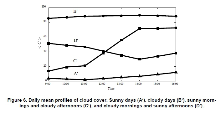
The diurnal variation in C is shown in Figure 6 as a plot of class mean <C> for the four classes.

3.5 Forecasting

As mentioned previously, two approaches were used to apply a cloud cover forecast to determine a B_nforecast. The first was to use the four classes of C obtained from clustering. For a given day, the C forecast was obtained; and the day was assigned to one of the C classes by finding the nearest centroid in the 8-d cluster space. The associated irradiance class was then regarded as the forecast of the irradi-ance class of that day. The forecast irradiance profile is the class mean profile, with estimated uncertainty given by the class standard deviation. For example, suppose that a given day is forecast to belong to C class A'. Then the irradiance forecast is that the day belongs to the associated class A.

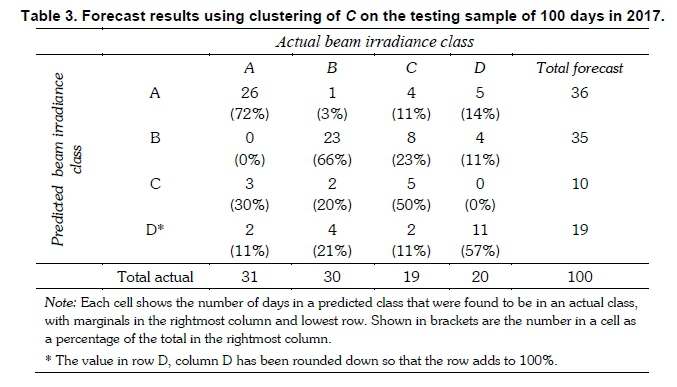
The forecasting results using the classes of C are presented in Table 3. Each cell in Table 3 shows the number of days in a predicted class that were found to be in an actual class, with marginals in the rightmost column and lowest row. Shown in brackets are the number in a cell as a percentage of the total in the rightmost column. For example, the first row shows the 36 days predicted to be in class A, of which 26 were in Class A, 1 in B, 4 in C and 5 in D. Thus 72% of days predicted to be in Class A were in Class A, whereas 3% were actually in Class B, 11% in C and 14% in D. The number of correct predictions is in the main diagonal.

Table 3 shows that prediction success rate per class ranges from 50-72%, with Classes A and B having the highest rates. Regarding incorrect predictions, predicted Class A was actually Class B for only one day (3%) and predicted Class B was actually Class A in zero cases. This is because, for a good NWP, it should be unusual for a sunny day to be wrongly forecast as a cloudy day and vice-versa. Classes C and D had a higher percentage of incorrect predictions, although Class D's success rate of 58% is not much lower than that of Class B. The success rate of 65% over all classes may only be applied to the period January to June from which the sample of 100 days was drawn, but it so happens that a standardised rate based on weighting with class frequencies over one year, given in Table 1, also gives a success rate of 65%.

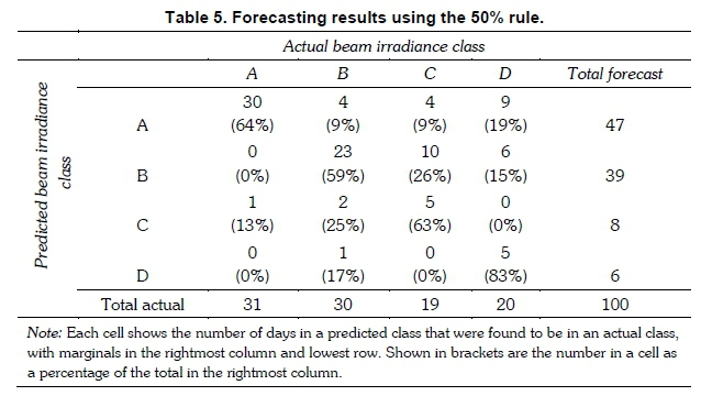
The second forecasting method uses a simple decision rule, termed the '50% rule' because it assigns a C profile to a class depending on whether the morning average (Cam) and afternoon average (C_PM) are above or below 50%. This method was chosen as a simple alternative to clustering that considers the diurnal variation of the B_nclasses. The 50% rule is described in Table 4.

 

 

The forecasting results using the 50% rule are presented in Table 5, which has the same format as that of Table 3.

Table 5 shows that the 50% rule produces prediction success rate per class in the range 59-83%, which is somewhat better than that of the C clustering forecast, except that there is a higher rate (9%) of Class B incorrectly predicted as Class A. The Class D success rate is significantly better, although the sample is rather small. Furthermore, Class D predicted by the 50% rule has only about a third of the days predicted to be in Class D by C clustering because, as may be seen in Figure 5, Class D' has a large number of days with C_AM < 50%, which are therefore predicted by the 50% rule to be in Class A. This increased the number of sunny (Class A) days predicted by the 50% rule. A consequence is that the 50% rule results in more Class A days being incorrectly predicted than in the C clustering method. In comparison with C clustering, the prediction success rate decreased for Classes A and B (by 8% and 7%, respectively) and increased for Classes C and D (by 13% and 25%). The overall raw success rate is 63%, and the standardised success rate is 64%, both of which, apart from being almost identical, are very close to that of the C clustering method.

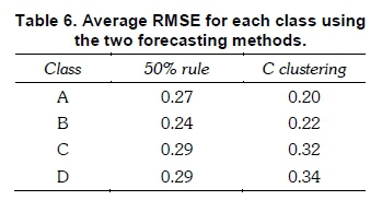
Table 6 shows the average RMSE values, computed using Equation 3, for each class using the respective forecasting method. Overall, the average RMSE per class are similar using the two forecasting methods, with smaller RMSE for Classes A and B using C clustering, and smaller RMSE for Classes C and D using the 50%rule. The largest difference is in Class A.

 

4. Discussion

Clustering one year of radiometric profiles (B_n) yielded four classes that describe diurnal patterns in Durban. It turned out that PCA applied to the 481-dimensional Bn (minute-resolution) profiles resulted in the same clusters obtained from B_n(hour-resolution), which indicates that hour-resolution profiles contain sufficient information for the four main clusters. These were very similar to four of the five classes obtained for Reunion Island by Jeanty et al. (2013) and Badosa et al. (2013). They were also similar to the three classes obtained by McCandless et al. (2014), of which the sunny (Class A) and cloudy days (Class B) formed two distinct classes whereas the partly cloudy days in the McCandless et al. (2014) classification were subdivided here by diurnal pattern into Classes C and D.

Two methods were tested to forecast daily beam irradiance profiles from cloud cover output of NWP: C clustering and the 50% rule. The forecasting results showed that the two methods produced comparable prediction success rates in the range 5083%. The overall success rates were about 65% for both methods, with variation for the different classes. The C clustering showed the best performance in predicting sunny days (Class A), followed by cloudy days (Class B). This may be due to the NWP model being able to distinguish between cloud-free and cloudy situations relatively well. By contrast, the 50% rule had a success rate that is better for the mixed conditions of Classes C and D. This may be due to the stronger separation of cloud cover conditions by the 50% rule as compared with clustering. Average profile error as quantified by RMSE was in the range 0.2-0.34. These results are similar to those of Badosa et al. (2015), where the lowest RMSE was for sunny conditions. However, in contrast to the present study where the highest RMSE where found for mixed conditions, Badosa et al. (2015) found the highest forecasting errors were associated with cloudy conditions. The main difference in the methods is that the present work used cloud cover output of NWP, with clustering of cloud cover profiles, and uses beam rather than global irradiance.

The novelty of this investigation is the use of clustering of cloud cover output from NWP, as well as the 50% rule, for day-ahead forecasts of beam irra-diance using classification of daily irradiance profiles. The forecasting methods have moderate success, which may be attributed both to the degree of accuracy of NWP and the existence of clusters of diurnal irradiance profiles, which show a high degree of clustering for sunny and cloudy conditions but are less well-clustered for mixed conditions.

 

5. Conclusions

Clustering of B_nfor Durban, South Africa, produced four classes with diurnal patterns as follows: sunny all day (Class A), cloudy all day (Class B), sunny morning and cloudy afternoon (Class C) and cloudy morning and sunny afternoon (Class D). These results provide a classification of beam irradiance profiles for Durban, and a novel approach to day-ahead forecasting using classification of cloud cover predictions, in particular by clustering. Day-ahead forecasts have value in predicting the general daily profile and are useful for constraining models for multi-hour predictions on a particular day. Further work that will be useful to better characterise irradiance patterns and produce day-ahead forecasts includes use of diffuse irradiance and sub-hourly variability of beam irradiance.

 

Acknowledgements

The authors would like to acknowledge Professor Miloud Bessafi, University of La Reunion, Electronic, Energy and Processes Laboratory, for his valuable discussions and guidance, and Mathieu Delsaut of the same institution for his assistance with clustering techniques. P. Govender thanks the South African National Research Foundation and Eskom's Tertiary Education Support Programme for financial support.

 

References

Aguiar, L.M., Pereira, B., Lauret, P., Dia z, F. and David, M. 2016. Combining solar irradiance measurements, satellite-derived data and a numerical weather prediction model to improve intra-day solar forecasting. Renewable Energy 97: 599-610. https://doi.org/10.1016/j.renene.2016.06.018        [ Links ]

Badosa, J., Haeffelin, M. and Chepfer, H. 2013. Scales of spatial and temporal variation of solar irradiance on Reunion tropical island. Solar Energy 88: 42-56. https://doi.org/10.1016/j.solener.2012.11.007        [ Links ]

Badosa, J., Haeffelin, M., Kalecinski, N., Bonnardot, F. and Jumaux, G. 2015. Reliability of day-ahead solar irradiance forecasts on Reunion Island depending on synoptic wind and humidity conditions. Solar Energy 115: 306-321. https://doi.org/10.1016/j.solener.2015.02.039        [ Links ]

Brooks, M.J., du Clou, S., van Niekerk, W.L., Gauche , P., Mouzouris, M.J., Meyer, R., van der Westhuizen, N., van Dyk, E.E and Vorster, F.J. 2015. SAURAN: A new resource for solar radiometric data in Southern Africa. Journal of Energy in Southern Africa 26(1): 2-10.         [ Links ]

Diabaté, L., Blanc, P. and Wald, L. 2004. Solar radiation climate in Africa. Solar Energy 76: 733-744.         [ Links ]

Gastón-Romeo, M., Leon, T., Mallor, F. and Rami rez-Santigosa, L. 2011. A morphological clustering method for daily solar radiation curves. Solar Energy 85, 1824-1836.         [ Links ]

Halkidi, M., Batistakis, Y. and Vazirgiannis, M. 2001. On clustering validation techniques. Intelligent Information Systems 17: 107-145. https://doi.org/10.1023/A:1012801612483        [ Links ]

Harrouni, S., Guessoum, A. and Maafi, A. 2005. Classification of daily solar irradiation by fractional analysis of 10-min-means of solar irradiance. Theoretical and Applied Climatology 80: 27-36. https://doi.org/10.1007/s00704-004-0085-0        [ Links ]

Ineichen, P. and Perez, R. 2002. A new airmass independent formulation for the Linke turbidity coefficient. Solar Energy 73: 151-157. https://doi.org/10.1016/S0038-092X(02)00045-2        [ Links ]

Inman, R.H., Pedro, H.T.C. and Coimbra, C.F.M. 2013. Solar forecasting methods for renewable energy integration. Progress in Energy and Combustion Science 39: 535-576. https://doi.org/10.1016/j.pecs.2013.06.002        [ Links ]

Jeanty, P., Delsaut, M., Trovalet, L., Ralambondrainy, H., Lan-Sun-Luk, J.D., Bessafi, M., Charton, P. and Chabriat, J.P. 2013. Clustering daily solar radiation from Reunion Island using data analysis methods. In: Proceedings of the International Conference on Renewable Energies and Power Quality (ICREPQ'13), Bilbao, Spain. https://doi.org/10.24084/repqj11.340        [ Links ]

Jolliffe, I.T. 2002. Principal component analysis. Springer, New York.         [ Links ]

Kunene, K., Brooks, M.J., Roberts, L.W. and Zawilska, E. 2013. Introducing GRADRAD: The greater Durban radiometric network. Renewable Energy 49: 259-262. https://doi.org/10.1016/j.renene.2012.01.019        [ Links ]

Lleti ', R., Ortiz, M.C., Sarabia, L.A. and Sanchez, M.S. 2004. Selecting variables for k-means cluster analysis by using a genetic algorithm that optimises the silhouettes. Analytica Chimica Acta 515: 87-100.         [ Links ]

Lorenz, E., Hurka, J., Heinemann, D. and Beyer, H.G. 2009. Irradiance forecasting for the power prediction of grid-connected photovoltaic systems. IEEE Journal of Selected Topics in Applied Earth Observations and Remote Sensing 2: 2-10. https://doi.org/10.1109/JSTARS.2009.2020300        [ Links ]

Lysko, M.D. 2006. Measurements and models of solar ir-radiance. PhD Thesis. Norwegian University of Science and Technology.         [ Links ]

Maafi, A. and Harrouni, S. 2003. Preliminary results of the fractal classification of daily solar irradiances. Solar Energy 75: 53-61. https://doi.org/10.1016/S0038-092X(03)00192-0        [ Links ]

MacQueen, J.B. 1967. Some methods for classification and analysis of multivariate observations. In: Proceedings of 5th Berkeley Symposium on Mathematical Statistics and Probability, University of California.         [ Links ]

Mathiesen, P., Collier, C. and Kleissl, J. 2013. A highresolution, cloud-assimilating numerical weather prediction model for solar irradiance forecasting. Solar Energy 92: 47-61. https://doi.org/10.1016/j.solener.2013.02.018        [ Links ]

McCandless, T.C., Haupt, S.E. and Young, G.S. 2014. Short term solar radiation forecasts using weather regime-dependent artificial intelligence techniques. In: Proceedings of the 12th Conference on Artificial and Computational Intelligence and its Applications to the Environmental Sciences: Applications of Artificial Intelligence Methods for Energy. Atlanta, Georgia.         [ Links ]

McCandless, T.C., Haupt, S.E., Young, G.S. and Annun-zio, A.J. 2015. A regime-dependent Bayesian approach to short-term solar irradiance forecasting. In: Proceedings of the13th Conference on Artificial Intelligence: Applications of Artificial Intelligence Methods for Energy-Part II. Phoenix, Arizona.         [ Links ]

Muselli, M., Poggi, P., Notton, G. and Louche, A. 2000. Classification of typical meteorological days from global irradiation records and comparison between two Mediterranean coastal sites in Corsica Island. Energy Conversion and Management 41: 1043-1063. https://doi.org/10.1016/S0196-8904(99)00139-9        [ Links ]

Perez, R., Moore, K., Wilcox, S., Renne, D. and Zelenka, A. 2007. Forecasting solar radiation: Preliminary evaluation of an approach based upon the national forecast database. Solar Energy 81: 809-812. https://doi.org/10.1016/j.solener.2006.09.009        [ Links ]

Remund, J., Perez, R. and Lorenz, E. 2008. Comparison of solar radiation forecasts for the USA. In: Proceedings of the 23rd European Photovoltaic Solar Energy Conference, Valencia, Spain.         [ Links ]

Rousseeuw, P.J. 1957. Silhouettes: a graphical aid to the interpretation and validation of cluster analysis. Journal of Computational and Applied Mathematics 20: 53-65. https://doi.org/10.1016/0377-0427(87)90125-7        [ Links ]

Sandia National Laboratories (SNL). 2012. Pv_lib toolbox for matlab.pvpmc.sandia.gov/applica-tions/pv_lib-toolbox/matlab/ [Accessed 30 August 2017].         [ Links ]

Soubdhan, T., Emilion, R. and Calif, R. 2009. Classification of daily solar radiation distributions using a mixture of Dirichlet distributions. Solar Energy 83: 1056-1063. https://doi.org/10.1016/j.solener.2009.01.010        [ Links ]

Zagouras, A., Inman, R.H. and Coimbra, C.F.M. 2014. On the determination of coherent solar microclimates for utility planning and operations. Solar Energy 102: 173-188. https://doi.org/10.1016/j.solener.2014.01.021        [ Links ]

Zawilska, E. and Brooks, M.J. 2011. An assessment of the solar resource for Durban, South Africa. Renewable Energy 36: 3433-3438. https://doi.org/10.1016/j.renene.2011.05.023        [ Links ]

Zhandire, E. 2017. Solar resource classification in South Africa using a new index. Journal of Energy in Southern Africa 28(2): 61-70. https://doi.org/10.17159/2413-3051/2017/v28i2a1640        [ Links ]

 

 

* Corresponding author: +27 31 260 1330; email: paulenegovender@gmail.com