ARTICLES

 

Wind power variability and power system reserves in South Africa

 

 

Poul Sørensen^{I, *}; Marisciel Litong-Palima^I; Andrea N. Hahmann^I; Schalk Heunis^II; Marathon Ntusi^III; Jens Carsten Hansen^I

^IDepartment of Wind Energy, Technical University of Denmark, Frederiksborgvej 399, 4000 Roskilde, Denmark
^IIEOH Energy Solutions & Analytics, Woodmead Estate, 1 Woodmead Drive, Woodmead 2191, South Africa
^IIIEskom, PO Box 1091, Johannesburg 2001, South Africa

 

 

---

ABSTRACT

Variable renewable generation, primarily from wind and solar, introduces new uncertainties in the operation of power systems. This paper describes and applies a method to quantify how wind power development will affect the use of short-term automatic reserves in the future South African power system. The study uses a scenario for wind power development in South Africa, based on information from the South African transmission system operator (Eskom) and the Department of Energy. The scenario foresees 5% wind power penetration by 2025. Time series for wind power production and forecasts are simulated, and the duration curves for wind power ramp rates and wind power forecast errors are applied to assess the use of reserves due to wind power variability. The main finding is that the 5% wind power penetration in 2025 will increase the use of short-term automatic reserves by approximately 2%.
Highlights
• Simulations are validated against observations of 30 minutes ramp rates.
• Absolute wind power ramp rates increase from 2014 to 2025.
• Normalised wind power ramp rates decrease from 2014 to 2025.
• Wind power will not impact the use of instantaneous reserves.
• Wind power will increase use of regulating reserves with less than 3% in 2025.

Keywords: variable generation; forecast errors; ramp rates; power curve estimation; fluctuations

---

 

 

1. Introduction

According to the Department of Energy (DoE), South Africa has taken off on a new trajectory of sustainable growth and development, illustrated by the growth of wind and photovoltaic (PV) generation from 48 GWh/m in January 2014 to 343 GWh/m in December 2014 [1]. For comparison, electricity consumption was 231 TWh/y in 2014 in South Africa [2]. Installed capacities were approximately 600 MW wind and 1000 MW PV by the end of 2014 [1]. This is the first step towards the implementation of the National Development Plan for 7 GW wind and solar to be commissioned by 2020, and a ministerial target of 13.2 GW by 2025 [1].

Wind and solar generation is variable, depending on the weather. International experience shows that increasing shares of variable generation adds uncertainty to the unit commitment and dispatch, on top of the load uncertainties and unscheduled outages of other plants in the power system. The development of large offshore wind farms was initiated in Denmark with the commissioning of the 160 MW Horns Rev wind farm in 2002. The experience of the owner, Elsam Engineering, with the operation of Horns Rev showed that placing many wind turbines in a small area would, in some cases, result in large minute-scale power fluctuations due to local weather situations [3], which is not the case for a similar capacity of wind turbines dispersed over a larger land area. For the same reason, the Danish transmission system operator (TSO) Energinet found that incorporating more wind power in the North Sea and maintaining the power balance in Western Denmark requires focusing on the necessary regulating power [4]. This resulted in developing and validating a model for wind power fluctuations, taking into account minute-range fluctuations and spatial correlations of wind speeds [5,6].

The importance of the location of wind farms in affecting spatial and temporal correlation was confirmed in the Minnesota Wind integration study [7]. In this study, the cost of additional reserves attributable to wind generation was assessed to be about USD 0.11/MWh of wind energy at 20% penetration by energy. Further, it was found that the expanse of the wind generation scenario, covering Minnesota and the eastern parts of North and South Dakota, provides for substantial 'smoothing' of wind generation variations. This smoothing is especially evident at time scales within the hour, where the impacts on regulation and load following were almost negligible. This confirms the importance of appropriate modelling of spatial and temporal correlations of wind power.

In countries with high shares of variable renewable generation, the uncertainty of variable generation and load is significantly reduced using forecast systems based on weather models and statistical models. The unit commitment and dispatch are usually scheduled before the day of operation, which introduces day-ahead forecast uncertainties. In the all-island grid study of wind variability management in Ireland, the need for replacement reserves was assessed based on the 90th percentile of the forecast error, which increased significantly with additional wind generation as well as forecast horizon [8]. This forecast uncertainty can be reduced using intraday balancing to update the unit commitment and dispatch schedule, but there will still be a need for reserves to balance generation and load at the time of operation, i.e., real time.

The present study analyses the variability and predictability of wind power generation and whether those characteristics of variable generation will have an impact on the need for reserves in the future South African power system. For this purpose, existing tools and methods were further developed, considering the existing practice and requirements in the system. Section 2 describes the simulation of meteorology time-series. The time-series were simulated using the Weather Research and Forecasting (WRF) mesoscale model run in a set-up validated in the Wind Atlas for South Africa (WASA) project [9], and they covered the entire country with 10 x 10 km² spatial resolution and one-hour temporal resolution. Section 3 describes the estimation of wind power curves based on historical data for wind power generation in existing wind power plants (WPPs). Those power curves provide the relation between WRF wind speeds and WPP power generation. They are different from the conventional wind turbine power curve published by manufacturers, firstly because of down-scaling and wake effect. Section 4 describes the simulation of wind power time series using the CorWind [10] software developed by the Technical University of Denmark: Department of Wind Energy (DTU Wind Energy). CorWind simulates wind power time-series with a higher temporal resolution than the WRF data. This software also simulates wind power forecast time-series consistent with the simulated wind power time-series. Section 6 describes the existing practice and requirements in South Africa's power system, focusing on reserve categories. Section 7 studies the impact of wind power fluctuations and forecast errors on the use of reserves. Section 8 concludes the study.

 

2. Simulation of mesoscale time-series

The meteorological time-series used in the present study is based on the down-scaling applied in the Wind Atlas for South Africa (WASA) project [11], but modified to include the entire country. Meteorological data was produced using a mesoscale reanal-ysis method, which is often used for obtaining highresolution climate or climate change information from relatively coarse-resolution global general circulation models or reanalysis [12]. The mesoscale reanalysis uses a limited-area, high-resolution model, which is driven by boundary conditions from the reanalysis. The strength in using the models to fill the observation gaps is that the fields are dynamically consistent; and they are defined on a regular grid. Additionally, the models respond to local forcing that adds information beyond what can be represented by the observations. The applied mesoscale reanalysis uses the National Centre for Atmospheric Research Advanced Research Weather Research and Forecasting model [13], version 3.5.1, released in September 2013. The model forecasts used 41 vertical levels from the surface to the top of the model located at 50 HPa; 12 of these levels are placed within 1000 m of the surface. The model setup uses standard physical parameterisations including the Mellor-Yamada planetary boundary layer scheme [14].

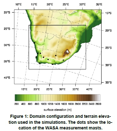
The model was integrated within the domains indicated by the rectangular shapes shown in Figure 1. The outer domain (1) has a horizontal spacing of 30 x 30 km². The inner domain (2) model grid has a horizontal spacing of 10 x 10 km², on a Lambert projection with centre at 29°N, 25°E. The domain has dimensions of 195 X 150 points.

 

 

The simulation covers 25 years (1990-2014) of meteorological time-series. Individual runs are re-initialised every 11 days. Each run overlaps the previous one by 24 hours to avoid using the time during which the model is spinning up mesoscale processes. A similar method was used and verified in other studies [11, 12, 15]. Initial and boundary conditions, and grids for nudging are supplied by the European Research Area interim reanalysis [16].

Sea surface temperatures (SSTs) that evolve with time and are derived from satellite and in situ measurements are also used in the simulation. These fields are at a horizontal resolution of 0.25° X 0.25° latitude vs. longitude [17]. They replace the coarse resolution SSTs available from the reanalysis (0.7° X 0.7°) and adequately represent the horizontal structure and time evolution of the SSTs in this area.

New output fields not available in the standard model were added to the simulation. These include hourly-averaged wind speed, hourly-averaged kinetic energy flux, and hourly-integrated solar insolation.

 

3. Estimation of power curves

The purpose of estimating power curves is to use them to simulate WPP generation time-series with WRF wind speed time-series as input. The estimated WPP power curves should, therefore, provide the relation between the wind speeds from the WRF model time-series and the WPP power generation at the same time. This is noteably different from conventional wind turbine (WT) power curves, which provide the relation between the wind speed in hub height close to the WT and the WT power. In principle, the relation between the WRF wind speeds and the WPP power could be obtained in two steps: downscale the WRF wind speeds to the location of all WTs in the WPP and, in that process, include the wake effects; then the WT power curves could be used in a second step with the downscaled wind speeds as input. Such a downscaling approach, however, requires detailed plans for WPP and WT siting. In addition to that, wind speed measurements would also be needed to obtain a sufficient accuracy for the downscaling for some sites. Therefore, an alternative approach is chosen, using observed wind generation time series recorded in the same period as the WRF data to estimate power curves. One year of observed generation time series (26 August 2014 - 25 August 2015) from eight WPPs was used to estimate the power curves. The temporal resolution of the observed time series is 30 minutes.

3.1 Methodology for estimating power curves

Figure 2 shows the scatter of simultaneous one-hour averages of WRF wind speed and measured power for a WPP. This scatter is very high compared with scatter of ten-minute averages used in WT power curves. The main reason for this difference is that the WRF wind speed time-series are modelled with meso-scale effects and resolution, whereas the measured WT wind speeds are measured close to the WT.

 

 

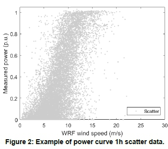
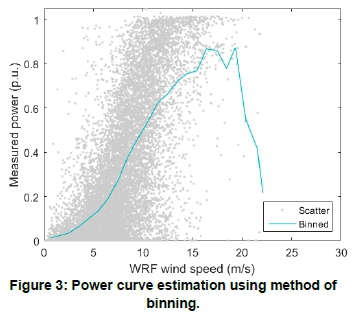
Figure 3 shows the estimated power curve using the standard method of bin, which is specified in the WT power curve standard IEC 61400-12-1 [18]. In short, this method first divides the wind speed axis into intervals or bins, then all pairs of wind speed/power data are sorted into the bins. Finally, the average wind speed and average power is calculated in each bin. The results showed that, with the present scatter, it is questionable to use this power curve. For instance, the maximum power is less than 0.9 per-unit (pu). for the binned power curve, although the maximum measured power is 1.0 pu. Using this power curve to simulate WPP power time series would result in an unrealistic probability distribution of the simulated power with maximum power values, which are much smaller than the maximum values of the measured power.

 

 

Alternatively, the power curve can be derived from the duration curves of WRF wind speeds and measured power respectively, as illustrated in Figure 4. The idea is to pair the wind speeds and powers with the same percentile. This is illustrated by the vertical line connecting the two curves in Figure 4. The intersection between the vertical line and the upper curve gives the wind speed which corresponds to the power defined by the intersection between the vertical line and the lower curve.

 

 

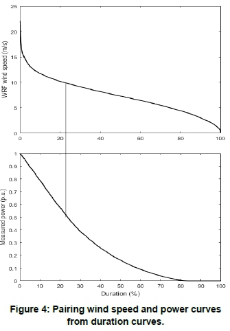
The advantage of the duration curve method is that the simulated wind power time series will have the same probability distribution as the original measurements. The main disadvantage is that this method assumes that the power curve is monotonic. Generally, this is a reasonable assumption for modern variable speed wind turbines with pitch control. However, the duration curve method neglects the decrease in power caused by shut downs of wind turbines at high wind speeds.

3.2 Wind farm power curves

In this section, specific power curves are first estimated for each of the eight WPPs with observed data. Then a general power curve is derived from the specific power curves. Figure 5 shows the specific power curves for each of the eight WPPs estimated with duration curve methodology. Generally, there are significant differences between the power curves, which illustrates the uncertainties associated with using a general power curve. The main objective for studying the use of fast reserves to deal with wind power variability is to get good accuracy in the sum of wind power from all WPPs in the system.

 

 

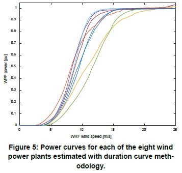
Two of the power curves are significantly lower than the other six. Since local conditions may explain this difference, a general power curve is determined as the average of the remaining six power curves.

 

4. Simulation of wind power time series

This section describes the simulation of wind power time series using CorWind software [10], which simulates wind power time series with a higher temporal resolution than the WRF data and provides wind power forecast time-series in addition to the real wind power generation time-series.

4.1 CorWind outputs and structure

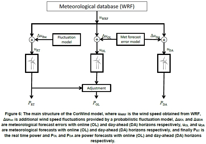
CorWind is an advanced tool developed at DTU Wind Energy for simulating wind power time series used in power system planning studies. It is capable of simulating consistent time-series of wind power production and prognosis. The main structure of CorWind is shown in Figure 6. It is based on a database of meteorological data, which is usually one-hour resolution data generated with WRF, as described in Section 2.

The left branch in Figure 6 provides the real-time wind power time-series PRT. In this context, real-time refers to the actual power, which is available at the time of operation, contrary to the forecasted powers. Mesoscale weather models like the WRF model generally underestimate the variability in the wind speeds [19]. In order to provide real-time wind speed time-series uRT with more realistic variability, CorWind adds fluctuations Aunuc to the WRF wind speeds u_WRF. The fluctuation model generation Au_fluc is further described in section 4.2.

CorWind uses power curves to convert wind speeds to power, and the simple power curve approach was extended with a method to include the shut-downs and start-ups caused by extreme weather conditions in the EU TWENTIES project [20][21].

The right branch in Figure 6 provides the day-ahead wind power time series Pda. It adds a wind speed forecast error Auda to uwrf to provide the day-ahead wind speed forecast uda before it is put through the wind-to-power conversion. Auda is generated using a multivariate autoregressive moving average (ARMA) process [22].

The middle branch in Figure 6 provides the online wind power forecast Pol. This is based on the same multivariate ARMA simulations, which were used to generate Δu_da, but uses the shorter horizon values compared with the day-ahead ARMA. The online forecast also includes an additional adjustment procedure, which ensures that the online forecast is improved on the basis of knowledge about the actually produced power, which is typically available to the TSO from the supervisory control and data acquisition (SCADA) of the energy management system.

4.2 Fluctuation model

The applied method in the fluctuation model, shown in Figure 6, is based on a frequency domain approach using power spectral densities (PSDs) to describe wind speed fluctuations and coherence functions to describe correlations [23]. The PSDs ensure a realistic fluctuation of the wind speed simulated in each point, while the coherence function ensures a realistic smoothening when the output power from several wind turbines or WPPs are added. The PSD Au_fluc must be calibrated to provide more realistic wind speed fluctuations of urt, in such a way that the PSD of u_rt matches the PSD of measured wind speeds. This calibration is performed based on wind speed measurements performed in the WASA project [24]. Since Au_fluc is generated as a random time series independent on uwrf, the relations between the PSDs can be expressed according to Equation 1.

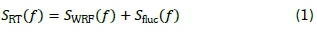
Figure 7 shows the PSDs S_meas(f) of measured wind speeds w_meas for ten masts in South Africa and for the PSDs S_vjRF(f) for the corresponding WRF wind speed 𝑤_WRF. Figure 7 confirms that there is a gap that starts around 2 x 10^-5 Hz between the measured and WRF PSDs because the WRF wind speeds underestimate the fluctuations.

 

 

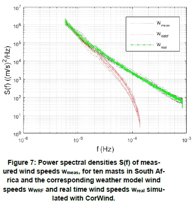
Larsen et.al. [25] showed that wind speed PSDs generally follow a - 5/3 power law for periods in the range of two hours to approximately 50 hours, which corresponds to frequencies in the interval from 6 x 10^-6 Hz to 10^-4 Hz. It can be observed from Figure 7 that S_meas(f) matches the - 5/3 power law very well for frequencies above 4 x 10^-5 Hz. CorWind uses S_flucc(f) as given in Equation 2 to ensure that the simulated S_RT (f) matches S_meas(f).

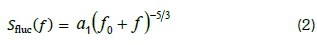
Assuming the high-pass cut-off frequency f₀ = 10^-5, the parameter a₁ = 5 χ 10^-4is estimated for the South African data. For comparison, a₁ = 3 χ 10^-4was estimated in the Danish offshore case [19]. This difference between the South African onshore and the Danish offshore cases can be translated to = 1.3 times larger amplitudes of the fast wind speed fluctuation components.

To verify the match between simulated and measured PSDs, Figure 7 also shows the PSDs S_RT(f) of the CorWind simulated wind speed w_real = w_RT which is seen to match 5_meas(f) very well.

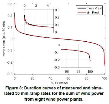
4.3 Validation

The one-year wind generation data used to estimate the power curves in Section 3, is now used to validate the ability of CorWind to simulate wind power time series with ramp rates that have probabilistic distributions close to the ramp rates of measured wind power time series. Figure 8 shows the duration curves of measured and simulated 30 min ramp rates for the sum of the 8 WPPs. The 30 min ramp rates are chosen for the comparison because the temporal resolution of the measured wind power time series is 30 min. Figure 8 shows a remarkable agreement between the measured and simulated ramp rate duration curves in the interval from 1 to 99%. In the low probability tails of the distributions, there are some deviations. It should be noticed that this very good result is obtained with the specific power curves estimated in Section 3 and the calibration of the fluctuation model in Section 4.2.

 

 

5. Time series statistics

This section presents the results of statistical analysis of the variability in the simulated wind power time series.

5.1 Simulation cases

Three simulation cases were defined in agreement with Eskom and DoE. Those cases are:

• 2014 being the reference (past) case including the WPPs installed in the beginning of the year;

• 2020 being the (planned) development case; and

• 2025 being a not too far future case to be considered in the grid development plans.

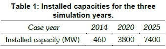
The total installed capacity for the 3 cases are shown in Table 1.

 

 

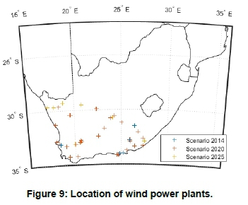
The location of the WPPs in each scenario is shown in Figure 9. The locations are affecting the correlations and thereby the spatial smoothening of the wind power fluctuations. For the 2014 and 2020 scenarios, the exact positions of the WPPs are known. For the additional WPPs in the 2025 scenario, the exact locations are not known at this stage, and therefore the locations of the expected connection points to the transmission system used.

 

 

5.2 Statistical analyses

The statistical analyses in this section are based on CorWind simulations of real wind power and wind power forecasts for the scenarios described in Section 5.1. The simulations of real wind power and of hour-ahead and online prognoses are done with five-minute temporal resolution, whereas the day-ahead forecasts are simulated with one-hour resolution, corresponding to the typical resolution of forecast systems. For the eight WPPs with historical data, the specific power curve for each WPP was used. For the remaining WPPs, the general estimated power curve was used. The simulations were done using all 25 years of WRF reanalysis time series. For each year, different random seeds are used to make the stochastic simulations in CorWind. This approach ensures a good coverage of annual as well as seasonal, diurnal and intra-hour variations. The wind power penetration of each scenario are shown in Table 2. The numbers were calculated assuming the 'SO moderate' 2020 and 2025 forecasts of electricity consumption according to the Integrated Resource Plan 2010-2030 [26].

 

 

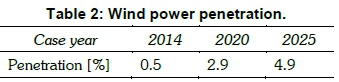
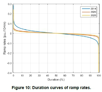
Figure 10 shows the duration curve of the ten-minute ramp rates for each of the scenarios. It illustrates that the pu (i.e. relative) ramp rates are reduced significantly from the 2014 to the 2020 scenario and further slightly reduced for the 2025 scenario. This is due to the smoothening effect with the WPP locations in Figure 9.

 

 

The smoothing effect is also distinct from the duration curves of forecast errors in Figure 11(a) (day-ahead) and (b) (hour-ahead).

 

 

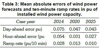
Table 3 summarises the mean absolute error of the forecast errors and ten-minute ramp rates for the different scenario years. The results show that the forecasts are improved, reducing the horizon from day-ahead to hour-ahead.

 

 

6. Reserve categories in South African power system

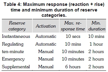
This section describes the different reserve categories in the power system. The South African ancillary services technical requirements [27] detail the requirements for different reserve categories and specifies five categories of reserves, as follows:

• instantaneous reserves - used to arrest the frequency within acceptable limits following a contingency;

• regulating reserves - used for second-by-second balancing of supply and demand, and under AGC control;

• the ten-minute reserves - to balance supply and demand for changes between the day-ahead market and real-time, such as load forecast errors and unit unreliability; and

• emergency reserves - used when the interconnected power system is not in a normal condition, and to return the system to a normal condition while slower reserves are being activated.

• supplemental reserves - used to ensure an acceptable day-ahead risk.

Table 4 shows a summary of requirements to response time (understood as reaction time plus rise time) based on the ancillary services technical requirements.

 

 

7. Assessment of needs for reserves

This section describes how the CorWind time series simulations were used to assess the use of reserves caused by wind power variability and prediction uncertainties.

7.1 Activation of reserve categories due to imbalances

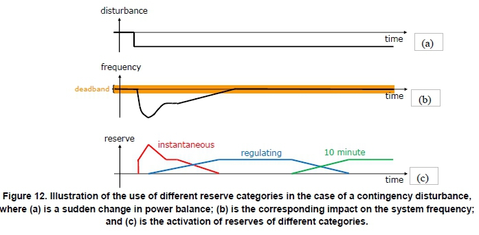
This section explains the impact of wind power on use of reserves by illustrating how the different reserve categories are activated and replaced in the case of load or wind power ramping, compared with the case of a contingency disturbance. Figure 12 illustrates the use of reserve categories in the case of a contingency disturbance: (a) is a sudden change in power balance caused by the contingency disturbance like tripping of a power plant; (b) is the corresponding impact on the system frequency; and (c) is the activation of reserves of different categories. The automatic instantaneous reserves respond fast to the frequency changes. The automatic regulating reserves also start to react fast to the imbalance, therefore reducing the frequency deviation and restoring the instantaneous reserves. Finally, in case of insufficient automatic reserves, the operator will manually activate ten-minute reserves to replace the automatic reserves.

In the case of load or wind power ramping, the use of reserves is different, as illustrated in Figure 13. Initially, the frequency will ramp down slower because the initial imbalance is quite small. With this small frequency change, the instantaneous reserves will not be activated, because the frequency is inside the dead band of the governor. Instead, the regulating reserves will balance the variation with a smalltime delay (12 seconds). Again, if the imbalance caused the available automatic reserves to be insufficient, the operator would manually activate ten-minute reserves to replace the regulating reserves.

 

 

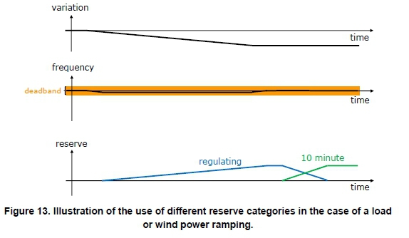
Observations from these illustrations suggest that the wind power variability is not affecting the use of instantaneous reserves. The following sections will, therefore, only describe the impact of wind power variability on regulating reserves and ten-minute reserves.

7.2 Influence of wind on regulating reserve requirements

According to the South African ancillary services technical requirements, regulating reserves should be sufficient to cover the genuine load variations within the hour. The present practice is to calculate the ten-minute load pickup and load drop-off to quantify the load variations. Moreover, the approximately 5% largest load variations are removed and the load variation is determined as the maximum of the remaining approximately 95%. This is done in order to not include the steepest deterministic (and therefore predictable) diurnal load variations.

Taking the impact of wind and other variable generation into account requires that the variations of the total (sometimes denoted residual) load should be considered, instead of the pure consumption. The total load is defined according to Equation 3.

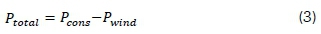
Equation 3 between power also applies to the corresponding ten-minute load pickup and load drop off, which is mathematically the same as the ramp rates used to quantify wind power variability in section 4. It is now assumed that the ten-minute ramp rates of wind power are uncorrelated with the ten-minute load pickup and load drop off. Then the relation between the standard deviations of the ramp rates becomes

The present practice and the need for regulating reserves are determined by the load variations, which are regularly analysed and updated by Eskom. In the present requirements, where variable generation is not considered, the approximately 95% load variations are varying between 400 and 650 MW [27].

If the ramp rate distributions were Gaussian, then the relation between standard deviations in Equation 4 would apply to any quantiles. For the present analysis, this is assumed to be approx-imately the case for the 95% quantile, i.e. as in Equation 5:

The 95% quantiles of the ten-minutes wind power ramp rates in Figure 10 are given in Table 5 for each scenario case year.

 

 

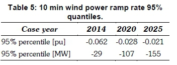
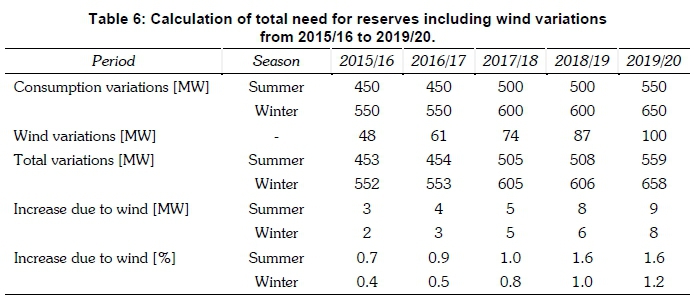
Table 6 (overleaf) shows the impact of wind power on the total need for reserves. The first two rows show the latest calculations of the reserves needed to cover the consumption variations from 2015/16 to 2019/20 [27]. The next line is the wind variations for each of the years, interpolating between the absolute value of the wind power quan-tiles from Table 5 in 2014 and 2020. Next, the total variations are calculated according to according to Equation 5. Finally, the increase due to wind is calculated as the difference between the total variations and the consumption variations, both in MW and in % of the original consumption variations. It is seen that the increased need for reserves is less than 10 MW and less than 2% in the entire 5-year period from 2015/16 to 2019/20.

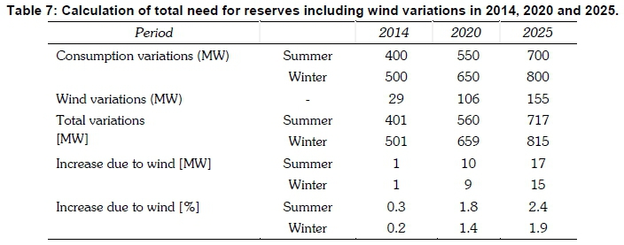
Table 7 (overleaf) shows the same calculations for the scenario case years. This was done by extrapolating the consumption variations using the pattern of the regulating reserve requirements in [27]. The impact of taking wind power into account is an increase of the requirements to regulating reserves with 1.8% in summer 2020 and 2.4% in summer 2025.

Since the consumption variations were given with 50 MW resolution, it is likely that the above calculated increases due to wind power would not have affected the result with this resolution. On the other hand, it would be good practice to include the impact of wind power variations in future updates of the technical requirements.

7.3 Influence of wind on ten-minute reserve requirements

Figure 13 shows that the ten-minute reserve will be activated to replace the regulating reserves shortly after they are activated. This brings the system back to a secure normal state with sufficient automatic reserves. The practice in Denmark is that power is traded day-ahead by the independent power producers (IPPs) on the common Nordic power exchange, Nord Pool. After the day-ahead trade, the balancing responsible IPPs can trade on the Elbas intra-day market. Finally, the Danish TSO Ener-ginet.dk plans the balancing on an hour-ahead basis using the Nordic Operation Information System list, which is a common Nordic regulating power list including bids from Danish, Norwegian, Swedish and Finnish market participants.

It is understood that the generation in South Africa is also scheduled day-ahead, which means that the day-ahead forecast error will have to be balanced. Balancing due to contingencies will typically be done as soon as possible during intra-day using supplemental reserves. It should, however, be noticed that early intra-day balancing based on updated wind power forecasts have a risk of being counterproductive if the balancing is done too early. Therefore, hour-ahead balancing is generally recommended for wind power forecast errors, but of course this must be assessed by the operator in the individual cases.

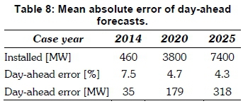
With the South African reserve categories from Section 6, most of the day-ahead wind power forecast errors will, therefore, be balanced by ten-minute reserves. Table 8 shows the mean absolute error of the day-ahead wind power forecasts, which must be balanced.

 

 

8. Conclusions

An application of the CorWind methodology to simulate correlated wind power time series was presented, where the simulations to assess the need for reserves in the South African power system was applied. This is a pilot application of the methodology, which includes validation of ramp rate statistics of simulated time-series against measured time-series. The main conclusions of the work are as follows: • The normalised day-ahead and hour-ahead forecast errors, as well as the ramp rates of wind power, will be reduced significantly from 2014 to 2020, and further reduced in 2025 because of the spatial smoothing.

• The expected wind power development in South Africa is expected to cover 2.9% of the electricity production in 2020 and 4.9% in 2025.

• Wind power variability will not influence the use of instantaneous reserves, because of the moderate rate of change of wind power combined with the frequency deadband.

• Wind power variability is estimated to increase the use of regulating reserves with a maximum of 1.8% in 2020 and a maximum of 2.4% in 2025; these numbers are less than the 50 MW resolution used in the South African technical requirements to ancillary services, but they may still have a minor impact on the future assessments of the need for regulating reserves.

• The use of ten-minute reserves is expected to increase to balance the day-ahead wind and photovoltaic power forecast errors; the wind power forecast errors were quantified in the present work, but the total need for ten-minute reserves was not studied.

 

Acknowledgements

The work was supported in part by the South African National Energy Development Institute under the contract for the project 'System adequacy and reserve margins with increasing levels of variable generation.'

 

References

[1] State of renewable energy in South Africa. Department of Energy, South Africa, 2015. http://www.gov.za/sites/www.gov.za/files/State%20of%20Renewable%20Energy%20in%20 South%20Africa_s.pdf.         [ Links ]

[2] Electricity generated and available for distribution (Preliminary). Statistical release P4141. Statistics South Africa, February 2015. http://www.statssa.gov.za/publications/P4141/P4141February2015.pdf.         [ Links ]

[3] Kristoffersen, J. R. The Horns Rev wind farm and the operational experience with the wind farm main controller. Offshore Wind International Conference, Copenhagen (2005).         [ Links ]

[4] Akhmatov, V., Abildgaard, H., Pedersen, J., Eriksen, P.B. Integration of offshore wind power into the Western Danish power system. Offshore Wind International Conference, Copenhagen (2005).         [ Links ]

[5] Sørensen, P. E., Cutululis, N. A., Vigueras-Rodriguez, A., Madsen, H., Pinson, P., Jensen, L., Hjerrild, J., Donovan, M. (2008). Modelling of power fluctuations from large offshore wind farms. Wind Energy, 11(1), 29-43. DOI: 10.1002/we.246. http://onlinelibrary.wiley.com/doi/10.1002/we.246/abstract.         [ Links ]

[6] Sørensen, P. E., Cutululis, N. A., Vigueras-Rodri-guez, A., Jensen, L.E., Hjerrild, J., Donovan, M., Madsen, H. Power Fluctuations From Large Wind farms. IEEE Transactions on Power Systems Vol 22 (3) (2007). http://ieeex-plore.ieee.org/documenf4282056/.         [ Links ].

[7] Zavadil R. et. al.. Final Report - 2006 Minnesota Wind Integration Study Volume I. Nov. 2006. EnerNex Corporation. https://www.leg.state.mn.us/edocs/edocs?oclcnumber=80967997.         [ Links ]

[8] Meibom, P., Barth, R., Brand, H., Hasche, B., Swider, D., Ravn, H., & Weber, C. (2008). All island grid study. Wind variability management studies. Dublin: Department of Enterprise, Trade and Investment. (Workstream 2B). http://www.eirgridgroup.com/site-files/library/EirGrid/ Workstream%202B.pdf.         [ Links ]

[9] Wind Aatlas for South Africa - http://www.wasaproject.info/ and http://wasa.csir.co.za/.         [ Links ]

[10] Sørensen, P. and Cutululis, N.A. Wind farms' spatial distribution effect on power system reserves requirements. 2010 IEEE International Symposium on Industrial Electronic (ISIE), 2010, Bari (IT), 4-7 July. http://ieeexplore.ieee.org/document/5636304/. DOI: 10.1109/ISIE.2010.5636304.         [ Links ]

[11] Hahmann A.N., Lennard C., Argent B., Badger J., Vincent C.L., Kelly M.C., Volker P.J.H., Refslund J., 2014b. Mesoscale modeling for the wind atlas for South Africa (WASA) Project. Technical Report, DTU Wind Energy, Roskilde, Denmark. http://orbit.dtu.dk/en/publications/mesoscale-modeling-for-the-wind-atlas-of-south-africa-wasa-project(8d6c8668-c38d-45a9-8640-18e069bf2c97).html.         [ Links ]

[12] Hahmann, A.N., Rostkier-Edelstein, D., Warner, T. T., Liu, Y., Vandenberg, F., Babarsky, R. and Swerdlin, S. P. A reanalysis system for the generation of mesoscale climatographies. Journal of Applied Meteorology and Climatology, 2010: 954-972. DOI: 10.1175/2009JAMC2351.1.         [ Links ]

[13] Wang, W., Bruyere, C., Duda, M., Dudhia, J., Gill, D., H-C. Lin, H-C., Michaelakes, J., Rizvi, S. and Zhang, X. WRF-ARW Version 3 Modeling System User's Guide. Mesoscale & Microscale Meteorology Division, National Center for Atmospheric Research, Boulder, USA, 2009. http://www2.mmm.ucar.edu/wrf/users/docs/user_guide_V3.7/ARWUsersGuideV3.7.pdf.         [ Links ]

[14] Mellor, G. L. and Yamada, T. Development of a turbulence closure model for geophysical fluid problems, Reviews of Geophysics and Space Physics, 1982: 851-875. http://www.fap.if.usp.br/~hbarbosa/uploads/Teaching/Mod-clim2010a/MellorYamada1982.pdf.         [ Links ]

[15] Hahmann, A.N., Vincent, C.L., Pena, A., Lange, J. and Hasager, C.B., Wind climate estimation using WRF model output: method and model sensitivities over the sea. International Journal of Climatology, 2014. DOI: 10.1002/joc.4217.         [ Links ]

[16] Dee, D.P. et al., The ERA-Interim reanalysis: configuration and performance of the data assimilation system. Quarterly Journal of the Royal Meteorological Society 2011: 553-597. DOI: 10.1002/qj.828.         [ Links ]

[17] Reynolds, R. W., Rayner, N. A., Smith, T. M., Stokes, D. C. and Wang, W. Q. An improved in situ and satellite SST analysis for climate. Journal of Climate, 2002: 1609-1625 DOI: 10.1175/1520-0442.         [ Links ]

[18] IEC 61400-12-1. Wind turbines - Power performance measurements of electricity producing wind turbines. Ed. 1.0. IEC Geneva 2017. https://webstore.iec.ch/publication/26603.         [ Links ]

[19] Larsén, X., Ott, S., Badger, J., Hahmann, A. and Mann, J. Recipes for correcting the impact of effective mesoscale resolution on the estimation of extreme winds. American Meteorology Society, 2012: 521-533. DOI: http://dx.doi.org/10.1175/JAMC-D-11-090.1.         [ Links ]

[20] TWENTIES project. Final Report. October 2013. https://windeurope.org/fileadmin/files/library/publications/reports/Twenties.pdf.         [ Links ]

[21] Cutululis, N., Altiparmakis, A., Litong-Palima, M., Detlefsen, N. and S0rensen, P. Market and system security impact of the storm demonstration in task-forces TF2. TWENTIES Deliverable D16.6. 2013. http://orbit.dtu.dk/en/publications/id(f725d379-984e-4693-81c1- 4be7b7cdd365).html.         [ Links ]

[22] Söder, L. Simulation of wind speed forecast errors for operation planning of multiarea power systems. International Conference on Probabilistic Methods Applied to Power Systems, Ames (2004). http://ieeexplore.ieee.org/document/1378776/.         [ Links ]

[23] Sørensen, P., Hansen A., and Rosas, P. Wind models for simulation of power fluctuations from wind farms. Journal of Wind Engineering & Industrial Aerodynamics, 2002: 1381-1402. http://www.sciencedirect.com/science/article/pii/S016761050200260X.         [ Links ]

[24] WRF wind power forecasts for South Africa. http://veaonline.risoe.dk/wasa/.         [ Links ]

[25] Larsen, M. F., Kelley, M. C. and Gage, K. S. Turbulence spectra in the upper troposphere and lower stratosphere at periods between 2 hours and 40 days. Journal of the Atmospheric Sciences, 1982: 1035-1041. http://journals.ametsoc.org/doi/abs/10.1175/1520-0469(1982)039%3C1035%3ATSITUT%3E2.0.CO%3B2.         [ Links ]

[26] Integrated resource plan for electricity 2010-2030 - Revision 2. Final report. South Africa Department of Energy. March 2011. http://www.en-ergy.gov.za/IRP/irp%20files/IRP2010_2030_Final_Report_20110325.pdf.         [ Links ]

[27] Ancillary services technical requirements 2015/16 - 2019/20. Rev. 1 ESKOM 28-10-2014. http://www.eskom.co.za/Whatwere-doing/AncilliaryServices/Documents/TechReq2015.docx.pdf.         [ Links ]

 

 

* Corresponding author: Tel: +45 2136 2766; email: posq@dtu.dk