ARTICLES

 

Predicting clear-sky global horizontal irradiance at eight locations in South Africa using four models

 

 

Evans Zhandire^*

University of KwaZulu-Natal, School of Engineering, Engineering Access, Howard College Campus, Durban 4041, South Africa

 

 

---

ABSTRACT

Solar radiation under clear-sky conditions provides information about the maximum possible magnitude of the solar resource available at a location of interest. This information is useful for determining the limits of solar energy use in applications such as thermal and electrical energy generation. Measurements of solar irradiance to provide this information are limited by the associated cost. It is therefore of great interest and importance to develop models that generate these data in lieu of measurements. This study focused on four such models: Ineichen-Perez (I-P), European Solar Radiation Atlas model (ESRA), multilayer perceptron neural network (MLPNN) and radial basis function neural network (RBFNN) models. These models were calibrated and tested using solar irradiance data measured at eight different locations in South Africa. The I-P model showed the best performance, recording relative root mean square errors of less than 2% across all hours, months and locations. The performances of the MLPNN and RBFNN were poor when averaged over all stations, but tended to show performance similar to that of the I-P model for some of the stations. The ESRA model showed performance that was in between that of the Artificial Neural Networks and that of the I-P model.

Keywords: clear-sky irradiance, Linke turbidity index, ESRA model, Ineichen-Perez model, artificial neural networks

---

 

 

1. Introduction

Solar radiation exhibits variation that depends on astronomical and weather factors. The astronomically-driven variation is predictable from well-established equations [1, 2]. In general, weather-induced variations are less predictable and result in long- and short-term solar irradiance fluctuations that can only be predicted in a statistical sense[1]. Clear-sky conditions, on the other hand, present atmospheric conditions that produce predictable effects on solar irra-diance. There is growing interest in models that predict clear-sky solar irradiance, which resulted in the development of many models that vary in complexity and accuracy of prediction [3-11]. A majority of these models predict broadband clear-sky irradi-ance, where the clear-sky atmospheric effects are accounted for by broadband attenuation parameters such as Linke-turbidity coefficient [12, 13] and Angstrom coefficient [14, 15]. Calibration of the models for local conditions involves an empirical process that computes the relevant broadband attenuation parameters using the clear-sky irradiance models backwards, with a selection of measured local clear- sky solar irradiance data as input [16].

It is also possible to generate clear-sky irra-diance from a set of astronomical and weather parameters using artificial neural networks (ANNs). The ANNs approximate the functional relationship between random input and output variables by learning from examples made up of historical data output and input variables [17]. Published applications of ANNs in the field of solar energy include time-series forecasting of solar radiation quantities [18-21] and other function approximation or regression models that map a set of input parameters like temperature into radiation quantities [22-26]. One major attraction of ANN methods is their ability to find relations between input and output even if the representation was intractable [19]. The ANN can, therefore, map a wide range of possible combinations of input or explanatory variables to a single desired output. This, however, does not underplay the importance of carefully selecting the variables. Koca et al. [26], for example, showed that different combinations of inputs affected the performance of ANN models that predicted global solar irradiation.

Solar energy is one of the promising sources of energy in South Africa. It is therefore important to investigate the performance of solar radiation models for South African conditions. A growing database of solar irradiance data from measurements by the Southern African Universities Radiometric Network (SAURAN) [27] provides opportunities to investigate and develop clear-sky models for South African conditions. The present investigation considered four models, two of which are semi-empirical broadband models: Ineichen-Perez (I-P) [10] and Euro pean Solar Radiation Atlas (ESRA) [11], which take Linke turbidity index, Earth-sun geometrical parameters and other geographical parameters as inputs.

These models have been extensively investigated in other regions outside South Africa where relative root mean square errors (rRMSE) of less than 10% were reported [9, 6, 5, 28]. The other two models considered in this investigation are ANNs based models, one a multi-layer perceptron neural network (MLPNN) and the other a radial basis function neural network (RBFNN). All four models were calibrated to predict horizontal clear-sky solar irradiance from similar inputs that carry information about location, time of day and year as well as atmospheric conditions. Model performance was investigated across eight different locations. The theoretical details of these models are discussed, followed by a methodology that describes data preparation and model evaluation criteria.

 

2. The clear-sky models

2.1 Ineichen-Perez model

One form of expressing the I-P model for global horizontal clear-sky irradiance (GHIclear) is found in Reno et al. [5] and is given by Equation 1.

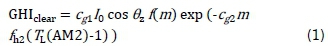
where:

• f(m) =exp(-c_g2m f_h1 + 0.01m¹⁸);

• f_h1=exp(-h/8000);

• f_h2=exp(-h/1250);

• c_g1 = 5.09x10^-5h + 0.868;

• c_g2 = 3.92x10^-5h + 0.0387

• T_L(AM2) is the Linke turbidity index evaluated at air mass, m = 2 or AM2;

• h is the station altitude in metres; and

• l₀ is the extraterrestrial solar irradiance at normal incidence, corrected for the eccentricity of the earth's orbit.

The air mass is computed from Equation 2, which was developed by Kasten and Young [29].

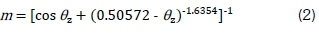
where θ_z is the apparent zenith angle.

2.2 European solar radiation atlas model

The GHI_clear for the ESRA model is given in Rigollier et al. [11] as the sum of beam horizontal clear-sky irradiance (BHI_clear) and diffuse horizontal clear-sky irradiance (DHI_clear). Equation 3 gives the expression for calculating the BHIclear.

where δ_R(m) is the Rayleigh optical thickness and its computation from air mass m is given by Kasten [13].

The diffuse irradiance on a horizontal surface, as shown by Equation 4, is expressed as a product a diffuse transmission function (Trd) and a diffuse angular function, (F_d).

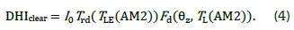
Detailed functional relationships T_rd(T_L(AM2)) and F_d(9_z, T_L(AM2)) are given in Rigollier et al. [11].

2.3 Artificial neural network models

General structure

A neural network model learns the statistical model that generates the data in a set of examples. The functional mapping of the model can be stated as in Equation 5.

where:

• x is a vector of inputs;

• w is vector of model parameters usually referred to as weights; and

• y is the model output.

During learning, the ANN optimises the weight matrix w so that the error between the desired output t, for input x, and the corresponding predicted output, y = y(x;w), is minimised. In ANNs that are applied to regression problems, the sum-of-squares error (SSE) function E is normally the preferred tar get objective [30]. Equation 6 defines E.

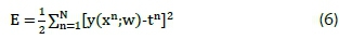
where n =1, 2,...N indexes the training patterns or features making up the training input matrix x, and the corresponding target output vector t.

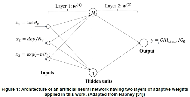
In this investigation, the ANN models estimate clear-sky global horizontal irradiance GHI_cl_earfrom three inputs.

Equations 7 and 8 define the model input and output variables.

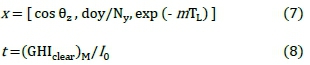
where:

• doy denotes the day of year number (it equals 1 for the first day of January);

• N_y, the number of days in a year; and

• (GHI_cl_ear)M is the target clear-sky irradiance selected from records of measured irradiance data.

Figure 1 shows the general form of the architecture of an ANN that implements this model.

The following sections give a more detailed account of the specific forms of the functional mapping of the MLPNN and RBFNN.

Multilayer perceptron neural network

Bishop [30] and Nabney [31] gave detailed descriptions of the functional mapping of a MLPNN. For a two-layer MLPNN with M hidden units, which maps three inputs to one output, the functional mapping can be written in the form of Equation 9.

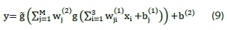
where:

• and represent the elements of the layer 1 and layer 2 weight matrices w⁽¹⁾and w⁽²⁾ respectively;

• and b⁽²⁾are bias parameters of the hidden and output units respectively;

• is input to the hidden unit j;

• g is a non-linear activation functio j gives Zj = ; and

• g is the activation function of the output unit, which can be linear, logistic sigmoidal or softmax.

The MLPNN is usually trained by the 'backpropagation method' [17], which optimises the input layer and output layer weights until a set objective (usually a set SSE) is achieved.

Radial basis function neural network

The RBFNN is considered as the main practical alternative to MLPNN for non-linear modelling [31]. The general radial basis function of the network mapping is given by Bishop [30] and Equation 10 specifies it to the three inputs and one output for the clear-sky model.

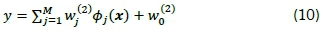
where:

• Wj are the elements of output layer vector of weights w⁽²⁾; and

• are basis functions, where the jth input data point X_jdefines the centre of the radial-basis function, and the vector x is the vector of inputs applied to the input layer [17]. Gaussian and thin plate spline function are some of the preferred basis functions in RBFNN.

Training of the RBFNN goes through a two-stage process. The first stage optimises the radial basis functions kernels, and stage two optimises the weight matrix of the output layer w⁽²⁾ by least squares method.

 

3. Methodology

3.1 Experimental

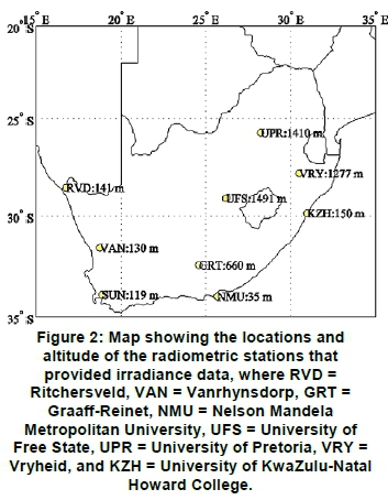
The irradiance information required for the calibrating and evaluation of the models was obtained from measurements performed by eight radiometric stations spread across South Africa, as shown in Figure 2. The stations form part of Southern African Universities Radiometric Network. Detailed information about the equipment used at the respective stations can be obtained from Brooks et al. [27] or by ac cessing the data portal webpage at http://www.sau-ran.net/.

 

 

3.2 Data preparation

Model inputs: The Linke turbidity indexes evaluated at air mass 2 (Tl(AM2)) can be computed from measured clear-sky direct normal irradiance (DNI) using Kasten's pyrheliometric formula, given as Equation 11.

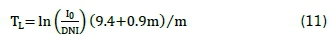
Using Equation 11, turbidity indexes limited to air mass in the range 1.99 < m < 2.2 were computed using yearlong samples of DNI data measured at each station. Linke turbidity indexes that fall out of a range defined by 2 < T_l< 5 were disregarded. This range was shown to be representative of clear skies for at least one location in South Africa [32]. The resulting time series of indexes were resampled, filtered and interpolated to produce yearlong time series of daily Linke turbidity indexes for each of the eight locations. The rest of the inputs, which include, solar zenith angle θ _ζ (φ, t), air mass m(G_z), and I₀, were all computed from well-known astronomical equations.

3.3 Model training and validation data.

The training patterns for the ANNs consisted of N X 3 input data matrix, x, as defined in Equation 7 and a corresponding output vector of N target elements t, as defined in Equation 8. The number of features, N, corresponds to the number of clear-sky GHI data points selected from one-minute averages of GHI data measured at the eight stations. The selection was according to a criterion defined by 0.97 < k_t < 1.01, where k_tis a clear-sky index calculated as a ratio of measured GHI to clear-sky GHI, given by the Ineichen-Perez model [10]. The training data were selected from measurements of GHI data gathered from 1 January 2014 to 31 December 2014.

Using the same criterion, the validation data for the all models were selected from a sample of GHI data measured from 1 January 2015 to 31 December 2015 at each of the eight stations.

3.3 Evaluation of model accuracy

The bias, precision, and accuracy of the models were evaluated from the following usual statistics. The relative mean bias error (rMBE) represents the mean bias of model prediction. Equation 12 defines the mathematical computation of the rMBE for the GHI_cl_earprediction models.

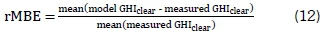
The rMBE gives an indication of how much a model under-estimates or over-estimates the observations. A sample of the model predictions may, however, consists of an even distribution of over-and under-estimated observations, resulting in the errors compensating each other and giving a false sense of unbiased predictions. The rRMSE gives a measure of the precision and bias or accuracy of the model. It is defined by Equation 13 for the GHI_clear prediction models.

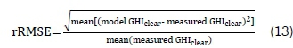
A potential drawback of rRMSE is its sensitivity to outlying estimates far away from the true value 33].

 

4. Results

4.1 Training and validation data

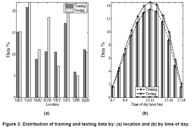
The training and testing data were derived from each of the eight stations. In plots (a) and (b) of Figure 3 the populations of the training and testing data, expressed as percentages of the total number of training sample data points N = 340 426, are plotted as functions of location and time of day, respectively. The contributions were not uniform, and show that University of Pretoria (UPR) and Vanrhynsdorp (VAN) contributed the least and largest amount of data, respectively. The hourly contributions were also not uniform, and followed a normal distribution centred about solar noon, as shown in Figure 3(b). The periods 6:00-7:00 and 17:0018:00 provided the least amount of training and validation data.

4.2 General performance of the models

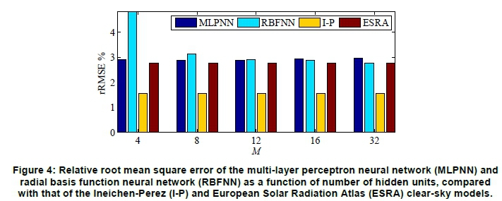
It is important to select the best possible network architectures for the ANN models. Since the number of inputs and the number of outputs were fixed at three and one respectively, the optimal architectures were determined by choosing the number of hidden units M that resulted in the least error. Architectures with 4, 8, 12, 16, and 32 hidden units were considered. Figure 4 shows the rRMSE averaged over all sites as functions of the number of hidden units for both the MLPNN and RBFNN models. The 3-12-1 architecture gave the best performance for the MLPNN, while the 3-32-1 architecture showed the best performance for the RBFNN. There was, however, a small difference between the performance of the 3-16-1 and 3-32-1 RBFNN architectures. A compromise between complexity and performance would thus favour the 3-16-1 RBFNN architecture. The results also reveal that the 3-16-1 RBFNN architecture performed better than the 3-12-1 MLPNN. Figure 4 also shows the performance of the I-P and ESRA models and reveals that these two models performed better that the ANNs models. The I-P model, with rRMSE < 2%, had the least prediction error.

4.3 Performance as a function of time

In Figure 5(a), the rRMSE is averaged over all locations and was plotted as a function of time of day for the 3-12-1 MLPNN, 3-16-1 RBFNN, I-P, and ESRA models. The ANNs and ESRA models showed similar trends where the rRMSE exhibited significantly larger errors during the early morning and late evening hours in comparison with a flat trend between 7:00 and 17:00. This contrasted with the trend exhibited by the I-P model that consistently performed with rRMSE below 2% for all the hours.

 

 

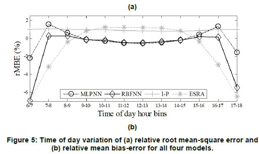
The prediction biases of the models are shown in Figure 5(b), where rMBE is plotted as a function time of day. Again, performance the I-P was consistent for all the hours of day, revealing a positive bias that indicated overestimation of the clear-sky GHI. The ESRA model also overestimated the GHI for the hours ranging from 9:00 to 15:00. The biases for the ANNs showed a similar trend with rMBE that was close to zero between 8:00 and 16:00. Given the large rRMSE, this trend suggests that the ANNs both overestimated and underestimated the GHI during this time interval, resulting in net-bias error that was close to zero.

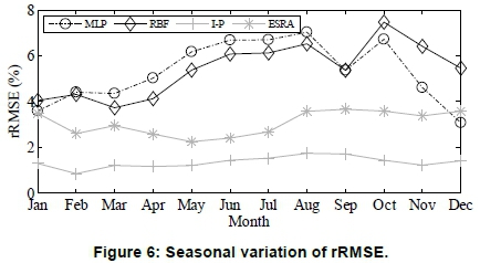
A further insight into variation of the performance of the models with time is shown in Figure 6, where rRMSE was plotted as a function of month of year. The performance of the ANNs varied the most with month of year and exhibited the largest monthly rRMSE. A comparison of the two ANNs models revealed that the RBFNN performed better than the MLP, except for the months of October to January. The I-P model also showed the most superior monthly prediction performance with rRMSE below 2% for all months.

 

 

4.4 Performance of the models across stations

Figure 7(a) and (b) show plots of the respective rMBE and rRMSE as functions of location or station.

 

 

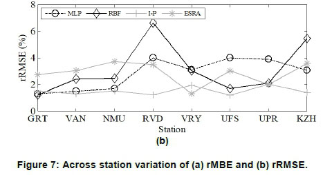
The results reveal that the I-P model produced the best performance at most of the stations. The performances of the ANNs, however, varied from being poor to closely matching the performance of the I-P model. A close match in performance amongst the three models was evident at the Graaff-Reinet, VAN

and Nelson Mandela Metropolitan University stations. This indicated poor generalisation that possibly resulted from overfitting of the dominating training patterns. The uneven distribution in the training patterns was noted in Section 4.1. The worst performance of the ANNs occurred at Ritchersveld.

In Figure 3(a), there was a disproportionately larger number of validation data compared with training examples. It was conceivable that the training data did not provide sufficient training examples to cover the range of the validation data.

4.5 Examples of clear sky GHI model predictions

Figure 8 illustrates a visual comparison of the models' predictions to the clear-sky GHI measured at Graaff-Reinet radiometric station. At the scale shown by the figures, the model predictions matched the measured clear sky GHI without perceptible differences, except for the hours close to solar noon. In these examples, the I-P model and the ANN models underestimated the clear-sky GHI at solar noon while the ESRA model produced the closest match.

 

5. Conclusions

This paper presented four models for predicting clear-sky global horizontal irradiance: Ineichen-Pe-rez (I-P), European Solar Radiation Atlas model (ESRA), multilayer perceptron neural network (MLPNN) and radial basis function neural network (RBFNN) models. The I-P model produced the most consistent and most accurate performance, recording relative root mean square errors (rRMSE) values of less than 2% across, all hours of day, all months of year and all locations. On the other hand, the two artificial neural networks (ANN) models, MLPNN and RBFNN, showed poor performance across all hours, and months for an all-stations-averaged evaluation. The evaluation of the ESRA model when averaged over all stations, hours and months revealed a performance that is close to that of the ANNs, recording rRMSE values of close to 3%. The performance of ANNs matched that of the I-P model for some of the stations, indicating that the ANNs 'remembered' the input and output relationships for these locations better, compared with other locations. It is, therefore, useful to explore ways to improve the generalisation capabilities of the ANNs for this clear-sky irradiance generation application.

 

Acknowledgements

The Southern African Universities Radiometric Network is thanked for providing solar radiation data.

 

References

1. Twidell, J. and Weir, T. 2006. Renewable energy resources, second edition, Taylor and Francis.         [ Links ]

2. Duffie, J. and Beckman, W. 2013. Solar Engineering of Thermal Processes, fourth edition, John Wiley and sons.         [ Links ]

3. Dai, Q. and Fang, X. 2014. A simple model to predict solar radiation under clear sky conditions. Advances in Space Research, 53: 1239-1245. http://dx.doi.org/10.1016/j.asr.2014.01.025.         [ Links ]

4. Badescu, V., Gueymard, C. A., Cheval, S., Oprea, C., Baciu, M., Dumitrescu, A., Iacobescu, F., Milos, I. and Rada, C. 2013. Accuracy analysis for fifty-four clear-sky solar radiation models using routine hourly global irradiance measurements in Romania. Renewable Energy, 55: 85-103. http://dx.doi.org/10.1016/j.renene.2012.11.037.         [ Links ]

5. Reno, M. J., Hansen, C. W. and Stein, J. S. 2012. Global horizontal irradiance clear sky models: Implementation and analysis. SANDIA report SAND2012-2389:        [ Links ]

6. Gueymard, C. A. 2012. Clear-sky irradiance predictions for solar resource mapping and large-scale applications: Improved validation methodology and detailed performance analysis of 18 broadband radiative models. Solar Energy, 86: 2145-2169. http://dx.doi.org/10.1016/j.solener.2011.11.011.         [ Links ]

7. Badescu, V., Gueymard, C. A., Cheval, S., Oprea, C., Baciu, M., Dumitrescu, A., Iacobescu, F., Milos, I. and Rada, C. 2012. Computing global and diffuse solar hourly irradiation on clear sky. Review and testing of 54 models. Renewable and Sustainable Energy Reviews, 16: 1636-1656. http://dx.doi.org/10.1016/j.rser.2011.12.010.         [ Links ]

8. Annear, R. L. and Wells, S. A. 2007. A comparison of five models for estimating clear-sky solar radiation. Water resources research, 43: 1-15. doi:10.1029/2006WR005055.         [ Links ]

9. Ineichen, P. 2006. Comparison of eight clear sky broadband models against 16 independent data banks. Solar Energy, 80: 468-478. http://dx.doi.org/10.1016/j.solener.2005.04.018.         [ Links ]

10. Ineichen, P. and Perez, R. 2002. A new airmass independent formulation for the Linke turbidity coefficient. Solar Energy, 73: 151-157. http://dx.doi.org/10.1016/S0038-092X(02)00045-2.         [ Links ]

11. Rigollier, C., Bauer, O. and Wald, L. 2000. On the clear sky model of the ESRA - European Solar Radiation Atlas - with respect to the heliosat method. Solar Energy, 68: 33-48. http://dx.doi.org/10.1016/S0038-092X(99)00055-9.         [ Links ]

12. Linke, F. 1922. Transmissions-koeffizient und Trübungsfaktor. Beitr. Phys. Fr. Atmos, 10: 91-103.         [ Links ]

13. Kasten, F. 1996. The linke turbidity factor based on improved values of the integral Rayleigh optical thickness. Solar Energy, 56: 239-244. http://dx.doi.org/10.1016/0038-092X(95)00114-7.         [ Links ]

14. Angstrom, A. 1929. On the atmospheric transmission of sun radiation and on dust in the air. Geo-grafiska Annaler, 11: 156-166. http://dx.doi.org/10.2307/519399.         [ Links ]

15. Louche, A., Maurel, M., Simonnot, G., Peri, G. and Iqbal, M. 1987. Determination of Angstrom's turbidity coefficient from direct total solar irradiance measurements. Solar Energy, 38: 89-96. http://dx.doi.org/10.1016/0038-092X(87)90031-4.         [ Links ]

16. Gueymard, C. A. Aerosol turbidity derivation from broadband irradiance measurements: methodological advances and uncertainty analysis. Solar 2013 Conference. Baltimore, MD, 2013.         [ Links ]

17. Haykin, S. 2009. Neural networks and learning machines, Third edition, Pearson Upper Saddle River, NJ, USA.         [ Links ]

18. Paoli, C., Voyant, C., Muselli, M. and Nivet, M.-L. 2010. Forecasting of preprocessed daily solar radiation time series using neural networks. Solar Energy, 84: 2146-2160. http://dx.doi.org/10.1016/j.solener.2010.08.011.         [ Links ]

19. Voyant, C., Notton, G., Kalogirou, S., Nivet, M.-L., Paoli, C., Motte, F. and Fouilloy, A. 2017. Machine learning methods for solar radiation forecasting: A review. Renewable Energy, 105: 569-582. https://doi.org/10.1016/j.renene.2016.12.095.         [ Links ]

20. Lauret, P., Voyant, C., Soubdhan, T., David, M. and Poggi, P. 2015. A benchmarking of machine learning techniques for solar radiation forecasting in an insular context. Solar Energy, 112: 446-457. https://doi.org/10.1016/j.solener.2014.12.014.         [ Links ]

21. Kashyap, Y., Bansal, A. and Sao, A. K. 2015. Solar radiation forecasting with multiple parameters neural networks. Renewable and Sustainable Energy Reviews, 49: 825-835. http://dx.doi.org/10.1016/j.rser.2015.04.077.         [ Links ]

22. Boznar, M. Z., Grasic, B., Oliveira, A. P. D., Soares, J. and Mlakar, P. 2017. Spatially transferable regional model for half-hourly values of diffuse solar radiation for general sky conditions based on per-ceptron artificial neural networks. Renewable Energy, 103: 794-810. http://dx.doi.org/10.1016/j.renene.2016.11.013.         [ Links ]

23. Hussain, S. and AlAlili, A. 2016. Online Sequential Learning of Neural Networks in Solar Radiation Modeling Using Hybrid Bayesian Hierarchical Approach. Journal of Solar Energy Engineering, 138: 061012-061012-10. http://dx.doi.org/10.1115/1.4034907.         [ Links ]

24. Chen, J.-L., Li, G.-S., Xiao, B.-B., Wen, Z.-F., Lv, M.-Q., Chen, C.-D., Jiang, Y., Wang, X.-X. and Wu, S.-J. 2015. Assessing the transferability of support vector machine model for estimation of global solar radiation from air temperature. Energy Conversion and Management, 89: 318-329. http://dx.doi.org/10.1016/j.enconman.2014.10.004.         [ Links ]

25. Lauret, P., Boland, J. and Ridley, B. 2013. Bayesian statistical analysis applied to solar radiation modelling. Renewable Energy, 49: 124-127. http://dx.doi.org/10.1016/j.renene.2012.01.049.         [ Links ]

26. Koca, A., Oztop, H. F., Varol, Y. and Koca, G. O. 2011. Estimation of solar radiation using artificial neural networks with different input parameters for Mediterranean region of Anatolia in Turkey. Expert Systems with Applications, 38: 8756-8762. http://dx.doi.org/10.1016/j.eswa.2011.01.085.         [ Links ]

27. Brooks, M. J., du Clou, S., van Niekerk, W. L., Gauché, P., Leonard, C., Mouzouris, M. J., Meyer, R., van der Westhuizen, N., van Dyk, E. E. and Vorster, F. J. 2015. SAURAN: A new resource for solar radiometric data in Southern Africa. Journal of Energy in Southern Africa, 26: 2-10.         [ Links ]

28. Engerer, N. A. and Mills, F. P. 2015. Validating nine clear sky radiation models in Australia. Solar Energy, 120: 9-24. http://dx.doi.org/10.1016/j.solener.2015.06.044.         [ Links ]

29. Kasten, F. and Young, A. T. 1989. Revised optical air mass tables and approximation formula. Applied optics, 28: 4735-4738. http://dx.doi.org/10.1364/AO.28.004735.         [ Links ]

30. Bishop, C. M. 1995. Neural Networks for Pattern Recognition, Clarendon Press.         [ Links ]

31. Nabney, I. T. 2002. NETLAB: Algorithms for pattern recognition., Great Britain, Springer.         [ Links ]

32. Sethabane, T. and Winkler, H. Atmospheric turbidity over Soweto. SAIP 2011, 2011. South Afica Institute of Physics, 525-530.         [ Links ]

33. Walther, B. A. and Moore, J. L. 2005. The concepts of bias, precision and accuracy, and their use in testing the performance of species richness estimators, with a literature review of estimator performance. Ecography, 28: 815-829.         [ Links ]

 

 

* Tel: +27 31 260 4101; email: Evans.zhandire@gmail.com