ARTICLES

 

Estimation of extreme inter-day changes to peak electricity demand using Markov chain analysis: A comparative analysis with extreme value theory

 

 

Caston Sigauke^{I, *}; Delson Chikobvu^II

^IDepartment of Statistics, School of Mathematical and Natural Sciences, University of Venda, Private Bag X5050, Thohoyandou, 0950, South Africa
^IIDepartment of Mathematical Statistics and Actuarial Science, Faculty of Natural and Agricultural Sciences, P.O. Box 339, Bloemfontein, 9300, South Africa

 

 

---

ABSTRACT

Uncertainty in electricity demand is caused by many factors. Large changes are usually attributed to extreme weather conditions and the general random usage of electricity by consumers. More understanding requires a detailed analysis using a stochastic process approach. This paper presents a Markov chain analysis to determine stationary distributions (steady state probabilities) of large daily changes in peak electricity demand. Such large changes pose challenges to system operators in the scheduling and dispatching of electrical energy to consumers. The analysis used on South African daily peak electricity demand data from 2000 to 2011 and on a simple two-state discrete-time Markov chain modelling framework was adopted to estimate steady-state probabilities of two states: positive inter-day changes (increases) and negative inter-day changes (decreases). This was extended to a three-state Markov chain by distinguishing small positive changes and extreme large positive changes. For the negative changes, a decrease state was defined. Empirical results showed that the steady state probability for an increase was 0.4022 for the two-state problem, giving a return period of 2.5 days. For the three state problem, the steady state probability of an extreme increase was 0.0234 with a return period of 43 days, giving approximately nine days in a year that experience extreme inter-day increases in electricity demand. Such an analysis was found to be important for planning, load shifting, load flow analysis and scheduling of electricity, particularly during peak periods.

Keywords: daily peak electricity demand; discrete time Markov chain; mean return time; transition probability matrix

---

 

 

1. Introduction

Forecasting of future extreme inter-day changes in electricity demand is important for proper planning in the dispatching and scheduling of electrical energy by system operators in the electricity sector. This calls for probabilistic modelling of the magnitude and time of occurrence of extreme positive inter-day changes in peak electricity demand. The use of Markov chains in probabilistic modelling and analysis of inter-day changes in peak electricity demand is not covered extensively in the literature. Some researchers, however, have used Markov chains and Markov decision processes in modelling electricity demand (McLoughlin et al., 2010; Widen and Wäckelgärd, 2010; Ardakanian et al., 2011; Haider et al., 2012; Sun and Li, 2014; Agyeman et al., 2015; among others). McLoughlin et al. (2010) modelled domestic load profiles using a Markov chain process and found that the magnitude of the load profile could be reproduced. A major shortcoming of this stochastic method for generating domestic load profiles was its inability to successfully model the time of peak loads during both day and night (McLoughlin et al., 2010). In a related study, a modelling framework for the stochastic generation of high-resolution data for occupant behaviour, presence, and energy use was published (Widén and Wäckelgärd, 2010) where nonhomogeneous Markov chains were used to create a spread of activities over time, up to the one-minute resolution. Empirical results from this study showed that the Markov chain model produced activity patterns that reproduced a spread of different end-use loads over time. Using a Markov chain analysis, Ardakanian et al. (2011) derived models for non-peak, off-peak and mid-peak periods in modelling home electricity consumption. Results from this study showed that the developed Markov chain models did not need more than six states, yet were accurate in transformer sizing in a distribution network. Markov models for predicting electricity demand are presented in Haider et al. (2012), where k-state models based on both discrete time and continuous time Markov chains were derived for different periods of the day. A comparative analysis was done with artificial neural networks and empirical results showed that the developed models produced accurate forecasts. Sun and Li (2014) estimated real-time electricity demand response of sustainable manufacturing systems using a Markov decision process and modelled the complex interaction and estimation of the potential capacity of demand reduction based on an automotive assembly line. Agyeman et al. (2015) used a variant of the hidden Markov model called a unsupervised disaggregation method, to detect the state of an appliance and its operation using household electricity meters. It was found that the developed model accurately provides power usage information which was important for demand-side response management.

Modelling daily peak electricity demand using the South African data is discussed in the literature (Sigauke et al., 2012; Sigauke et al., 2013; Verster et al., 2013; among others). Sigauke et al. (2012) developed a hybrid model called an autoregressive moving average - exponential generalised auto-regressive conditional heteroscedasticity - generalised single Pareto (ARMA-EGARCH-GSP) model for estimating extreme quantiles of inter-day increases in peak electricity demand. It was argued that this modelling approach captures the conditional heteroscedasticity in the data and can be used to estimate extreme tail quantiles of the distribution of the inter-day increases in peak electricity demand. A comparative analysis was done with an ARMA- EGARCH model, which showed that the ARMA-EGARCH-GSP outperformed the ARMA-EGARCH model in estimating extreme tail quantiles. Sigauke et al. (2013) also modelled extreme daily increases in peak electricity demand using generalised Pareto distribution (GPD) and performed a comparative analysis with the GSP distribution. Results showed that both distributions were a good fit to the daily increases in peak electricity demand data, but the use of the GSP distribution was found to be advantageous over the GPD because of having only one parameter to estimate, compared with two for the GPD. A detailed discussion on the policy implications of the study was then given. In a related study, Verster et al. (2013) used the GSP distribution in modelling the same day of the week upsurges in peak electricity demand. The parameters of the distribution were estimated using Bayesian inference (Beirlant et al., 2004) and maximal data information prior was used in this study. The GSP distribution was then used for estimating future exceedance probabilities and extreme tail quantiles. Subsequently, a comparative analysis was done with the GPD.

This investigation presents a Markov chain analysis of inter-day changes to peak electricity demand using South African electricity data, where inter-day changes were defined as daily increase/decrease in daily peak electricity demand. The niche of this is modelling of extreme positive inter-day changes in peak electricity demand using discrete time Markov chains (DTMCs), as a departure from existing literature. Such large changes pose challenges to system operators in the scheduling and dispatching of electrical energy to consumers. They are usually attributed to extreme weather conditions and the general random usage of electricity by consumers. Steady-state probabilities, including mean return times and first passage probabilities, were calculated for the inter-day changes in peak electricity demand. The investigation focused on extreme increases in electricity demand. Examples of similar interests are in the meteorology field and include: Why model average rainfall for a country when it is extremely heavy rainfall that causes a flood and destroys crops? Extremely low rainfall would cause drought, hence is more attractive to study than average rainfall. Sometimes there is a need to move away from the average thinking and concentrate more on the tails of distributions of electricity demand.

Section 2 presents the models, and empirical results are presented and discussed in Section 3. Section 4 presents a discussion of the results while Section 5 concludes.

 

2. Methodology

An inter-day change in peak electricity demand using a Markov chain is modelled in this investigation, with an approach of a DTMC problem with a finite state space given the stationary series in Figure 2(b). Initially, two states were defined: positive inter-day changes (increase) and negative inter-day changes (decrease). A transition matrix was developed and steady-state probabilities of the two states were then calculated with inclusion of mean return times and first-passage probabilities. A steady-state probability when reached is that, after a very long time, the distribution becomes constant and equal to the stationary distribution. The probability of an inter-day increase in electricity demand becomes a constant regardless of the last state occupied. The probability of an inter-day decrease in electricity demand becomes a constant regardless of the last state occupied. The two-state problem was then extended to a three-state problem by splitting the positive inter-day changes to small and extreme inter-day changes. This was done by fitting a nonparametric extremal mixture model to the positive inter-day changes to determine a sufficiently high threshold, with observations above this threshold being regarded as extreme positive inter-day changes and those below as small inter-day changes. The negative inter-day changes were treated as a third state, which was a decrease. A transition matrix was developed and a stationary distribution established. The focus was on the steady-state probability of extreme positive inter-day changes to find the first passage probabilities.

2.1 Description of the data

South African daily peak electricity demand (DPED) data for the period 1 January 2000 to 31 August 2011 was used, where Z₁,Z_Nwas considered to be a sequence of inter-day changes in peak electricity demand. The increase/decrease in peak demand is relative to the previous day (Sigauke et al., 2012). Let y_tbe equal to DPED on day t and y_t-1DPED on day t - 1, then the inter-day change, z_t, in peak electricity demand on day t, can be defined as in Equation 1.

Extreme large inter-day increases in peak electricity demand pose challenges to system operators of power utility companies that have to ensure grid stability by balancing supply and demand of electricity.

The time-homogeneous Markov chain analysis using the data for the sampling period, years 2000 to 2011, became the focus. It was with full recognition that electricity demand is also subject to other factors and drivers such as economic conditions, availability and capacity of the power system to meet the demand because of planned and unplanned outages, load shedding, coal shortages, among others, including price changes (Hyndman and Fan, 2010; Munoz et al., 2010; among others). This was, however, not considered in this investigation.

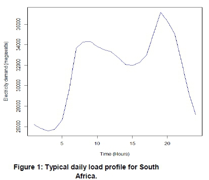
Figure 1 shows a typical daily load profile for the South African data. Large increases in electricity demand occur in the morning and in the evening.

 

 

Plots of DPED, inter-day changes in DPED, including density and box plots of inter-day changes in peak electricity demand are given in Figure 2. Figure 2(b) shows that DPED is made stationary by taking the first difference, defined as the inter-day change in peak electricity demand. Figures 2(c) and 2(d) suggest the presence of extreme increases in electricity demand.

2.2 Time-homogeneous discrete-time Markov chains

The transition probabilities of an inter-day increase or inter-day decrease of DPED is assumed to depend only on the current state (which is either a decrease (d) or an increase (i)) and not on past history of inter-day changes in DPED. If the probabilities for the future values of a discrete time, discrete state space process [Y_n n> 0} are dependent only on the latest available value, such a stochastic process has the Markov property and is called discrete time Markov chain (DTMC) (Kulkarni, 2011). Mathematically, a process {Y_n , n> 0} with discrete time set { η =0, 1,2, 3,...} and a discrete state space { d and i}, is given by Equation 2.

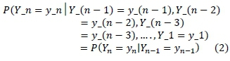
where y_nwill either be an increase or a decrease in DPED for η = 0,1,2,3 ...

A DTMC is said to be time-homogeneous if, for all η = 0,1,2,3 Equation 3 stands.

Equation 3 implies that, for time-homogeneous DTMCs, the one-step transition probability depends on m and j but is the same at all times n; hence the terminology time-homogeneous. The values m and j would each take a decrease(d) or increase(i).

The time-homogeneous DTMC Ρ is a time-invariant probability distribution; in fact, the chain considered here is stationary (or reaches steady state) (Kulkarni, 2011). This means that the statistical properties of the process remain unchanged as time elapses; see Figure 2(b) on inter-day changes in DPED. The statistical properties refer to probabilities, expected values, and variances. A stationary process will be such that over a given length of the time period for years, say, 2000 to 2002, will be statistically the same as the same length time period, e.g. 2006 to 2008.

2.3 Estimation of transition probabilities (inter-day changes)

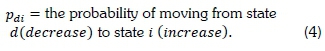
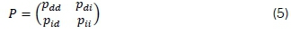
The transition matrix Ρ is a square M by M matrix, where M is the number of states S. The methods which are usually used for estimating the transition probabilities are maximum likelihood (ML), ML with Laplace smoothing, and the bootstrap approach (Spedicato et al., 2015). The transition probabilities are defined by Equation 4. Let:

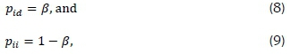
The other state probabilities are similarly defined; thus the transition probability matrix is defined by Equation 5, which can be broken down according to the series of Equations 6-11.

Differently, let

Then

Similarly, if

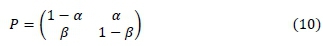
the transition probability matrix can be expressed according to Equation 10.

The state probabilities p_diare estimated by the method of maximum likelihood given by Equation 11.

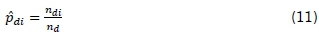
where, n_diis the observed number of transitions from state d to state i and is the observed number of transitions from state d. The other state probability estimates are similarly calculated.

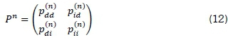
In the time-homogeneous case, the η -step transition probability of moving from one state to another state in exactly η steps can be calculated. The η-step transition probabilities for these states are given by Equation 12.

A derivation of the recursive equations is given in the supplementary material.¹

An irreducible, aperiodic Markov chain with a finite state space will settle down to its unique stationary distribution in the long run. A Markov chain is said to be irreducible if every state can be reached from every other state (Kulkarni, 2011). Two-state and three-state models are considered, which are therefore finite, where all states communicate and hence an irreducible chain and where the chain is not periodic. A state is said to be periodic with period D if a return to the same state is possible only in a number of steps that it is a multiple of D (Kulkarni, 2011).

2.4 Mean return time

The mean return time (T_i ), which is also known as the mean recurrence time of an ergodic (aperiodic and positive recurrent) Markov chain, is the expected first return time fi; for state I given by Equation 13.

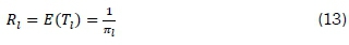
where π = (π₁,..., π _Μ ) is the stationary probability vector of P, and M is the number of states. The proof of the E(Ji ) is given in the supplementary information file. Mean return time gives the time in days), that if the current state is say an increase, the amount of time before another increase occurs.

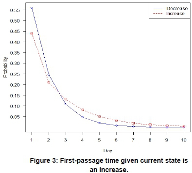
2.5 First-passage probability in states

One of the questions of interest is: How long will the current wave of the day upon day increase last? The problem can be formulated as: When will the stochastic process representing the inter-day change in the DPED move from the increase state to a decrease state? Such questions lead us to the study of the first-passage time (FPT), i.e., the random time at which a stochastic process first passes into a given subset of the state space.

The FPT is the number of steps, T_ly, taken by the Markov chain to arrive at state y for the first time given the initial state I (Feres, 2007). The probability distribution of the FPT is described by Equations 14-19 (Feres, 2007).

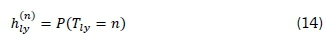
and

Now for η = 1,

and for n> 2

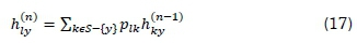
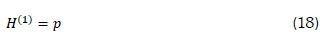
where S is the state space. If Hⁿdenotes the FPT matrix with entries and H_Oⁿdenotes the same FPT matrix with zeros on the diagonal entries, Feres (2007), then for η = 1 the result is given by Equation 18.

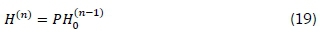
and for η > 1 the result is given by Equation 19.

where the (Zy)-entry denotes the probability of getting at state y for the first time at time η given the initial state I.

2.6 Modelling extreme peaks for the two- state problem

A nonparametric extremal mixture model, discussed in Scarrott and Hu (2015), is fitted on the positive inter-day changes so as to determine a sufficiently high threshold, τ. Observations above the threshold are then defined as extreme inter-day positive changes (state 1) and state 2 for observations less than or equal to τ, i.e z_t< τ. The cumulative distribution function of the nonparametric extremal mixture model (Scarrott and Hu, 2015) is given by Equation 20.

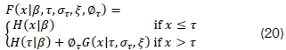
The bulk model is represented by H(. |.) with β denoting the bulk parameter, τ the fixed threshold, σ _τ and ξ denoting the scale and shape parameters respectively of the GPD fitted to the upper tail of the distribution, i.e. to observations above the threshold τ. The probability of an exceedance is represented by 0_T. A kernel density is fitted to the bulk model and a GPD to observations above τ. The parameters are then estimated using the maximum likelihood method.

2.7 The three-state problem

The two-state problem (decrease (d) and increase (i)) is then extended to a three-state problem. The positive inter-day changes are split into two states, which are small and extreme positive inter-day changes. The three states are formally defined by Equation 21.

for positive inter-day changes. The three states are: State 1: Observations between 0 and τ (small increase), i.e. (0 < z_t< 2838 MW), where MW = megawatts.

State 2: Observations above τ (extreme increase), i.e. z_t> 2838 MW, given by Equation 22.

 

for negative inter-day changes and will be zero for all of them.

State 3: Observations below zero (decreases in peak electricity demand, i.e. z_t< 0).

 

3. Results

Using the R statistical package 'Markovian' developed by Spedicato et al. (2015), the steady-state probabilities (for decrease and increase states) are π = (π _ά , π _ί ) = (0.5978,0.4022).

The mean return times for the two states are for the increase state: 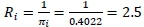days and for the decrease state

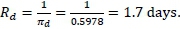
This shows that if the current state is an increase then another increase is expected in about two and half days. There should be 146 inter-day increases in DPED in a given year.

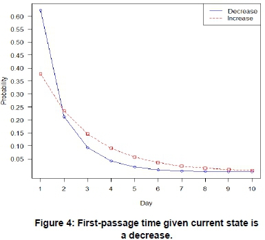
3.1 First-passage time probabilities

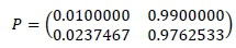
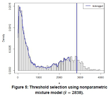
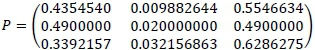
The first-passage times are represented by Figure 3, which shows that the graphs of the decrease and increase states intersect at about 2.5 days. Similarly, Figure 4 shows that the two curves intersect at about 1.7 days. Figure 5 shows a plot of threshold selection using a non-parametric extremal mixture model where a kernel density is fitted to the bulk model and a GPD fitted to the tail of the distribution with τ = 2838. The transition matrix for the two states: state 1: extreme increases (observations above τ), and state 2: no extreme increase (observations below τ), was found to be

 

 

 

 

 

 

and the steady-state probabilities were

The mean return times for the two states were

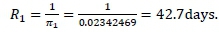
The extreme increase state, i.e. z_t> 2838 MW gives approximately nine days in a year of extremeincreases and 1day for the state z_t< 2838 MW.

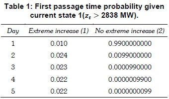
Table 1 shows that if the current state was 1 (z_t> 2838 MW), then the probability that the next day will have an extreme increase in peak electricity demand would be 0.01 while that of state 2 (no extreme increase) would be 0.99. The probability of state 2 decreases exponentially, while that of state 1 slowly increases. The first passage time probability given current state is 2 (z_t< 2838 MW) and is given in the supplementary material.

 

 

The probabilities of the three-state were found to be after computing.

Since the Markov chain is aperiodic and irreducible, the steady-state probabilities are: π = (π₁, π₂, π₃) = (0.3792457; 0.02342469; 0.5973296).

The mean return times are 2.6, 42.7 and 1.8 days for the three states. For the small increase state (0 < z_t < 2838) and for the extreme increase state (z_t>2838MW) as well as for the decrease state (z_t < 0).

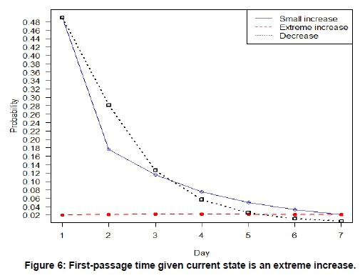
From the stationary distribution in Equation 12, the steady-state probability of an extreme increase was very small, 0.02342469, i.e. about 2.3% of the time an extreme positive inter-day change in peak electricity demand in South Africa is expected, while for about 60% of the time a decrease is expected. Table 2 shows that if the current state is a small increase there is a greater chance of a decrease the following day. If the current state were an extreme increase, then the chances of a small increase or a decrease are equally likely the following day as shown in Table 2.

 

 

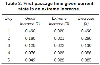
Figure 6 shows the first-passage time and the corresponding probabilities for the state extreme increase. Similar graphs for the other states are given in the supplementary material.

 

 

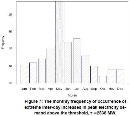
3.2 Monthly frequency of occurrence of extreme inter-day increases in peak electricitydemand

There are 101 observations above the threshold of 2838 MW (exceedances) over a period of 12 years (years 2000 to 2011) giving an average of nine (after rounding up) exceedances per year. The bar chart of the monthly frequency of occurrence of 101 extreme inter-day increases in peak electricity demand above the threshold of 2838 MW for the period 1 January 2000 to 31 August 2011 is given in Figure 7. This gives an average of nine extreme inter-day increases per year. This is consistent with the Markov chain analysis discussed in Section 3. Extreme large increases in inter-day changes in peak electricity demand are likely to occur in May, as shown in Figure 7. This could be due to the movement from summer to winter in the southern hemisphere.

 

 

4. Discussion

Markov chain analysis of inter-day changes in peak electricity demand using South African data has been discussed and applied in modelling frequency of occurrences of daily peak electricity demand. This analysis was extended by using nonparametric extremal mixture models. The threshold was determined using a nonparametric extremal mixture model in which a kernel density to the bulk model was fitted and a generalised Pareto distribution was fitted to the upper tail of the distribution. Parameters of this nonparametric extremal mixture model were estimated using the maximum likelihood estimation method.

From the Markov chain analysis, the steady state probability of an extreme increase (z_t > 2838 MW) in daily peak electricity demand was calculated to be 0.0234. This resulted in a mean return time of about 43 days. That is if the current state is an extreme increase another extreme increase is expected in about 43 days. This implies nine days in a year of extreme increases. The extreme increases are more likely to occur in May of every year. Results from the frequency analysis using extremal mixture models showed that there are 101 extreme inter-day increases in peak electricity demand above the threshold of 2838 MW for the period 1 January 2000 to 31 August 2011. The results were found to be consistent with those from the Markov chain analysis in that an average of nine extreme inter-day increases per year is experienced.

The analysis done in this paper potentially helps system operators and decision makers in power utility companies such as Eskom in South Africa to understand the stochasticity of peak electricity demand, and extreme inter-day changes. In a constrained power system such as that of South Africa, which is currently operating with a very tight reserve margin, the modelling approach also guides system operators in managing the risk of unplanned outages and the resultant inconvenience to consumers. Electricity demand is also subject to other factors and drivers such as economic conditions, availability and capacity of the power system to meet the demand, due to planned and unplanned outages, load shedding, coal shortages, among others including price changes.

 

5. Conclusions

The paper discussed an application of discrete time Markov chain analysis in modelling the frequency of occurrences of extreme daily peak electricity demand using South African data. A comparative analysis was then done with using the extreme value theory techniques in which a sufficiently high threshold was determined using non-parametric extremal mixture models. A kernel density was fitted to the bulk model and a generalised Pareto distribution to the tail distribution, i.e. to observations above the threshold.

 

Note

1 Supplementary data material with derivations and some of the tables and plots can be found at http://journals.assaf.org.za/jesa/rt/suppFiles/2329/0.

 

Acknowledgments

The authors acknowledge the National Research Foundation of South Africa (Grant No: 93613) for funding this research and Eskom for providing the data.

 

References

Agyeman, K.A., Han, S. and Han, S. Real-time recognition non-intrusive electrical appliance monitoring algorithm for a residential building energy management system. Energies, 2015, 8: 9029-9048.         [ Links ]

Ardakanian, O., Keshav, S. and Rosenberg, C. Markovian models for home electricity consumption, Proceedings of the 2nd ACM SIGCOMM workshop on Green networking, 2011: 31-36.         [ Links ]

Beirlant, J., Goedgebeur, Y., Segers, J. and Teugels, J. Statistics of extremes: Theory and applications, 2004, London, UK: Wiley.         [ Links ]

Feres, R. Notes for Math 450 Matlab listings for Markov chains, 2007. [online] http://www.math.wustl.edu/~feres/Math450Lect04.pdf (accessed 13 August 2016).         [ Links ]

Ferro, C.A.T. and Segers, J. Inference for clusters of extreme values. Journal of the Royal Statistical Society. Series B, Statistical Methodology, 2003, 65(2): 545 556.         [ Links ]

Haider, M.K., Ismail, A.K. and Qazi, I.A. Markovian models for electrical load prediction in smart buildings. In: Huang T., Zeng Z., Li C., Leung C.S. (eds) Neural information processing. ICONIP 2012. Lecture notes in computer science, 2012, Vol. 7664. Springer, Berlin, Heidelberg.         [ Links ]

Hyndman RJ, Fan S. Density forecasting for long-term peak electricity demand. Institute of Electrical and Electronics Engineers Transactions on Power Systems, 2010, 25(2):1142-1153.         [ Links ]

Kulkarni, V.G. Introduction to modelling and analysis of stochastic systems, 2011, Second edition, Springer, New York.         [ Links ]

McLoughlin, F., Duffy, A. and Conlon, M. The generation of domestic electricity load profiles through Markov chain modelling: 3rd International Scientific Conference on Energy and Climate Change; Conference proceedings: Athens, Greece, 2010, 18-27.         [ Links ]

Munoz, A., Sanchez-Ubeda, E.F., Cruz, A. and Marin, J. Short-term forecasting in power systems: a guided tour. Energy Systems, 2010, 2:129-160.         [ Links ]

Scarrott, C. J., Hu, Y. Evmix: Extreme value mixture modelling, threshold estimation and boundary corrected kernel density estimation, 2017. [online] http://www.math.canterbury.ac.nz/~c.scarrott/evmix (accessed 7 February 2016).         [ Links ]

Sigauke, C., Verster, A., Chikobvu, D. Tail quantile estimation of heteroskedastic intraday increases in peak electricity demand. Open Journal of Statistics, 2012: 435-442.         [ Links ]

Sigauke, C., Verster, A. and Chikobvu, D. Extreme daily increases in peak electricity demand: Tail-quantile estimation. Energy Policy, 2013, 53:90-96.         [ Links ]

Smith, L.R. Statistics of extremes, with applications in environment, insurance and finance, 2003. [online] http://www.stat.unc.edu/postscript/rs/semstatrls.pdf (accessed 16 March 2016).         [ Links ]

Spedicato, G.A., Kang, T.S and Yalamanchi, S.B. R package markovchain, version 0.4.3: 2015. [online] https://cran.r-project.org/web/packages/markovchain/markovchain.pdf (accessed 2 February 2016).         [ Links ]

Sun, Z. and Li, L. Potential capability estimation for realtime electricity demand response of sustainable manufacturing systems using Markov decision process. Journal of Cleaner Production, 2014, 65: 184-193.         [ Links ]

Verster, A., Chikobvu, D.and Sigauke, C. Analysis of the same day of the week increases in peak electricity demand in South Africa. ORiON, 2013, 29 (2): 125-136.         [ Links ]

Wide N, J. and Wäckelgard, E. A high-resolution stochastic model of domestic activity patterns and electricity demand. Applied Energy, 2010, 87: 1880-1892.         [ Links ]

 

 

* Corresponding author: Tel: +27 15 962 8135; email: caston.sigauke@univen.ac.za