


Serviços Personalizados
Artigo
 Inglês (pdf)
 Artigo em XML
 Referências do artigo
Indicadores

Links relacionados
-
 Citado por Google
 -
 Similares em Google
Compartilhar

 Permalink
Journal of Energy in Southern Africa
versão On-line ISSN 2413-3051
versão impressa ISSN 1021-447X
J. energy South. Afr. vol.28 no.4 Cape Town Nov. 2017
http://dx.doi.org/10.17159/2413-3051/2017/v28i4a2428
ARTICLES
Forecasting medium-term electricity demand in a South African electric power supply system
Caston Sigauke
Department of Statistics, School of Mathematical and Natural Sciences, University of Venda, Private Bag X5050, Thohoyandou 0950, South Africa
ABSTRACT
The paper discusses an application of generalised additive models (GAMs) in predicting medium-term hourly electricity demand using South African data for 2009 to 2013. Variable selection was done using least absolute shrinkage and selection operator (Lasso) via hierarchical interactions, resulting in a model called GAM-Lasso. The GAM-Lasso model was then extended by including tensor product interactions to yield a second model, called GAM-te-Lasso. Comparative analyses of these two models were done with a gradient-boosting model to act as a benchmark model and the third model. The forecasts from the three models were combined using a forecast combination algorithm where the average loss suffered by the models was based on the pinball loss function. The results showed significantly improved accuracy of forecasts, making this study a useful tool for decision-makers and system operators in power utility companies, particularly in maintenance planning including medium-term risk assessment. A major contribution of this paper is the inclusion of a nonlinear trend. Another contribution is the inclusion of temperature based on two thermal regions of South Africa.
Keywords: elastic net, generalised additive models, Lasso, tensor product interactions.
1. Introduction
Medium-term electricity demand is important to decision-makers in power utility companies in tactical planning for things such as generation capacity and maintenance planning, including medium-term risk assessment. Literature focuses mainly on forecasting short-term electricity demand (Gaillard et al., 2016; Fasiolo et al., 2017). Additive quantile regression models for forecasting both short-term probabilistic load and electricity prices for the Global Energy Forecasting Competition of 2014 (GEFCom2014) were discussed in Gaillard et al. (2016). The proposed new methodology of Gaillard et al. (2016) ranked first in both tracks of the competition. This methodology was extended by Fasiolo et al. (2017), where the development of fast calibrated additive quantile regression models for short-term load forecasting was done. Short-term forecasts are important to system operators in scheduling and dispatching electricity to meet demand. These forecasts are also important for the management of grid stability and load-flow analysis. On the other hand, planning for capacity development, including reserve margins, requires long-term point and probabilistic forecasts.
Whilst point forecasting focuses on predicting single observations, probabilistic forecasting gives the full distribution of the forecasts, which is more useful as it captures uncertainties in the forecasts (Hyndman and Fan, 2010). A review of probabilistic electric-load forecasting models is discussed by Hong and Fan (2016), where reviews on techniques and methodologies are given. The techniques are grouped under multiple linear regression models, semi-parametric additive models, artificial neural networks, exponential smoothing models, autoregressive moving average models, support vector machine, and fuzzy regression models, including gradient-boosting models. Hong and Fan (2016) also found that most of these techniques are applied to a larger extent to short-term and also, to a lesser extent, to long-term load forecasting. A summary of the probabilistic forecasting methods which were used in the GEFCom2014 are given in Hong et al. (2016).
Modelling electricity demand in South Africa has been published (Debba et al., 2010; Sigauke and Chikobvu, 2012; Sigauke et al., 2013). Using the Council for Scientific and Industrial Research sectoral regression model, Debba et al. (2010) presented forecasts for electricity demand in South Africa for 2010-2035. Using an additive regression model, Sigauke and Chikobvu (2012) discussed the modelling and forecasting of short-term electricity demand using South African data, where the developed model produced forecasts with mean absolute percentage error below 2%. Sigauke et al. (2013) discussed modelling of extreme daily increases in peak electricity demand using South African data, where focus was on tail quantiles of the distribution of daily peak electricity demand. It was found that such a modelling framework allows decision-makers to assess accurately the magnitude and frequency of occurrences of peak electricity demand. In all these cases variable selection methods are not discussed.
Temperature is known to be one of the major drivers of electricity demand (Hyndman and Fan, 2010; Munoz et al., 2010). Using South African data, Chikobvu and Sigauke (2013) assessed the influence of temperature on average daily electricity demand, using two references of 18 °C and 22 °C. These reference temperatures were determined using the multivariate adaptive regression splines (Friedman, 1991). It was found that, for temperature values above 22 °C, there are slight marginal increases in electricity demand, while for temperature below 18 °C demand increases significantly.
Application of statistical learning techniques such as generalised additive models (GAMs) in forecasting electricity demand in South Africa is not discussed in literature to the best of the author's knowledge. GAMs were developed by Hastie and Tibshirani (1990). Pierrot and Goude (2011) proposed the use of GAMs to forecast French hourly load data for over five years, and a comparative analysis was done with the operational model used by the French power utility. Variables in the developed GAM model included weather conditions, economic growth, weekly and yearly seasonality. Results from this study showed that the proposed model performs better than the operational one. A generalised additive modelling framework was proposed by Goude et al. (2014) to model electricity demand in France on 2260 sub-stations across the country, on both short- and middle-term horizons. Empirical results from this study showed good performance in both cases, i.e. short-term and middle-term forecasting. It was also shown that this modelling approach is capable of capturing big and complex datasets without human intervention; e.g., the load data used was collected over 2260 sub-stations for every ten minutes. Hyndman and Fan (2010) developed a semi-parametric additive model that is in the regression framework to forecast long-term peak electricity demand. Variables included in the developed model are calendar effects, price changes, and economic growth, including temperature effects. Empirical results from this study showed that the semi-parametric additive model provides accurate forecasts of the Australian half-hourly electricity demand.
In regression-based models, variable selection is important as it helps to reduce the dimension of the problem, while at the same time avoiding overfitting. The study used the least-absolute shrinkage and selection operator (Lasso) developed by Tibshirani (1996). Lasso is a regression method commonly used in variable selection in regression-based models. The Lasso is one of the shrinkage methods that include ridge regression and elastic net. It uses the penalty  . An extension is the elastic net (Zou and Hastie, 2005), which is a compromise between Lasso penalty
  and ridge regression penalty
  . Another extension of this is the grouped Lasso (Yuan and Lin, 2006; Meier et al., 2008), in which variables are included or excluded in the regression model in groups. There are a few cases in literature where Lasso has been used in regression-based models for electricity demand forecasting (Takeda et al., 2016; Ziel, 2016; Ziel and Liu, 2016). Using the ensemble Kalman filter and shrinkage multiple regression models, Takeda et al. (2016) developed a modelling framework for electricity load forecasting. The developed methodology was also used for analysis of the load structure. The proposed models outperform existing state space models. Ziel (2016) used a Lasso-based algorithm for estimating the autoregressive moving average-generalised autoregressive conditional heteroscedasticity (ARMA-GARCH) model to forecast hourly German electricity load. A bivariate time-varying threshold autoregressive model was developed and used by Ziel and Liu (2016) in probabilistic forecasting of load data from the Global Energy Forecasting Competition 2014 (GEFCom2014). The developed model outperformed two benchmark models from the competition, which were among the top eight entries of GEFCom2014.
For regression models with multiple seasonali-ties, interactions are important (Simpson, 2014; Xie et al., 2016; Laurinec, 2017). Electricity demand exhibits multiple seasonalities ranging from daily to weekly to monthly. Xie et al. (2016) developed models for probabilistic long-term electricity demand forecasting using both high resolution and low-resolution data. The resolutions of the data were hourly, daily and monthly. All the hourly demand models included interaction effects, referred to as cross-effects. Results from this study showed that models that use high-resolution data generally outperform those that use low-resolution data for both monthly peak and average monthly probabilistic forecasts. Simpson (2014) discussed an application of GAMs for seasonal time series data, using Central England temperature data. The models discussed capture the trend and seasonal variation, including interaction of the trend and seasonal features of the seasonal time series data. An application of generalised additive models with tensor product interactions in forecasting electricity consumption was discussed in Laurinec (2017). Empirical results from this study showed that the inclusion of tensor product interactions significantly improves the forecast accuracy. Wheeler (2017) proposed a Bayesian additive basis tensor product modelling framework for modelling high-dimensional surfaces. The developed model was applied to both simulated and reallife data. The new proposed modelling framework successfully linked chemical properties to predictions of dose-response patterns. Wood (2017) discussed a modelling framework that uses p-splines with derivative-based penalties and tensor product smoothing. It was found that such a modelling approach allows a choice of using either derivative-based or discrete penalties.
In the present study, GAM models with pairwise tensor product interactions were developed and used for medium-term forecasting of hourly electricity demand using South African data. Variables were selected using Lasso. The best GAM model with pairwise tensor interactions was compared with one without interactions. The two GAM models were then compared with a gradient-boosting model, which was used as a benchmark model. A major contribution of this paper is the inclusion of a nonlinear trend. Another contribution is the inclusion of temperature based on two thermal regions of South Africa.
Current research focuses mainly on the application of GAMs that were first developed by Hastie and Tibshirani (1986; 1990) and applied to load forecasting. The models, including the tensor interactions and variable selection using Lasso, are discussed in Section 2. Empirical results are presented and discussed in Section 3, while Section 4 draws conclusions.
2. Methodology
2.1 Generalised additive models
Let ythbe electricity demand on day t at hour h, where t = 1,η and h = 1, ...,24 with the corresponding covariates xthi, xth2, - , xthp, where ρ represents the number of variables. The generalised additive model is then written as in Equation 1.

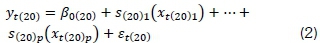
where ß0h is a constant parameter, shj are smooth functions and ethare independent and identically distributed error terms and are assumed to be auto-correlated. Electricity demand data for hour 20:00, i.e., h = 20, is modelled in this study, while it should be noted that this modelling approach can be applied to other times of the day. It therefore follows that the model is given by Equation 2.
Equation 1 is estimated using penalised cubic splines (Wood, 2006; Goude et al., 2014), which is expressed in terms of Equation 3.
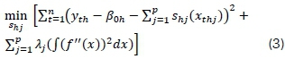
The degree of smoothness is controlled by the penalty parameter Λ = (Xj, j = 1,p), which determines the roughness of the function estimate to the data. It is optimised using the generalised cross-validation criterion (GCV) and easily implemented in the package 'mgcv' (Wood, 2006; 2017). For small values of Äj, the smoothness is rough. The smooth function, shj is given by Equation 4, which can be explained as the sum of basis functions, bhi(x) and their regression coefficients ßhi.

where q denotes the basis dimension. This study also uses p-splines, including cyclic (periodic) cubic splines to smooth the calendar effects, i.e., day of the week and month of the year.
2.2 Variable selection
The Lasso is used for variable selection (Tibshirani, 1996; Friedman et al., 2017) by constraining the absolute values of the coefficients of the model given in Equation 5.

where, ß0hand ßhj are parameters to be estimated and the other variables are as defined in Equation 1. Using Lasso, the estimates of ßhj are:  = argmin
 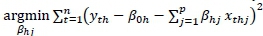 subject to
  That is, if the sum of the absolute values of the coefficients were below some predetermined value , the sum of the squared differences would be minimised. Constraining the sum of the magnitudes of the coefficients only means that important covariates will be included in the model, while the least important ones will be excluded, as they will be shrunk to zero (Friedman et al., 2017). The Lagrangian form of the Lasso formulation is given in Equation 6.
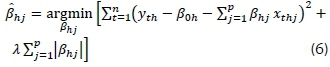
where λ is the shrinkage factor, which is 0 - 1 and is given by
Variable selection using Lasso will be done using the r package 'glmnet' developed by Friedman et al. (2017).
2.3 Tensor interactions
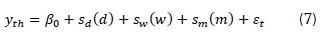
Considering the GAM model given in Equation 1, it is assumed that there are three covariates representing calendar effects, i.e., daily (d), weekly (w) and monthly ( ). This reduces Equation 1 to Equation 7.
Now, considering the smooth functions, sd, swand smof each of the three covariates, daily, weekly and monthly effects, the corresponding bases can be written as: I
 and
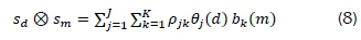
and  with λ}, Υι and ßkbeing parameters, and 9j(d), at(w) and bk (m) the spline basis functions (Wood, 2006). The tensor product of sdand sm, for example, is given by Equation 8.
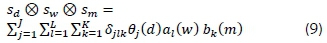
where  is the Kronecker product. Similarly, the tensor product of sd, swand smis given by Equation 9.
Tensor product smooths are known to be useful for representing functions of covariates measured in different units and are invariant to a rescaling of its covariates (Wood, 2006; Laurinec, 2017). Only pairwise tensor product interactions were considered in this study. Three functions in the 'mgcv' r statistical package (Wood, 2017) were also used for the definition of tensor product smooths and interactions. The functions are 'te , which is known to produce full tensor product smooths, 'ti' the function that produces hierarchical tensor product interactions, and 't2', which uses a penalisation method different from 'te' (Wood, 2006; Laurinec, 2017).
2.4 The generalised additive-tensor product interactions model with autocorrelated errors
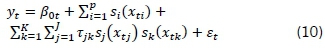
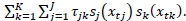
Let ytbe electricity demand at 20:00, i.e. yt = yt(20) as defined in Section 2.1, which gives the generalised additive model with pairwise tensor product interactions of autocorrelated errors as Equations 10 and 11.

where 0(B) is the nonseasonal autoregressive operator, θ (Β) is the nonseasonal moving average operator and the corresponding seasonal autoregressive and seasonal moving operators are Φ(Β) and Θ(Β) respectively; vtdenotes a white noise series. By expressing Equation 10 in terms of etand substituting in Equation 11, Equation 12 is produced.
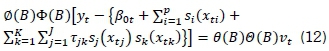
This study only considered cases where j ≠ k, i.e. where quadratic interactions are excluded. The total number of variables, i.e., main effects and interaction variables is: 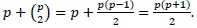 .
.
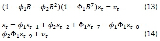
In practice, the challenge is the number of lags one should start off with for the model in Equation 11. Hyndman and Athanasopoulos (2013) proposed the following model for seasonal models SARIMA(2,0,0) X (1,0,0)[s], which is SARMA(2,0) X (1,0)[s], where s is the seasonal length. For this study s = 7, leads to the model expressed by Equation 13, which can be written as Equation 14.
From Equation 14, let 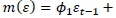
 and from Equation 10
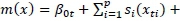
 . Equation 14 then leads to Equation 15.

Subsequently, Equation 10 reduces to Equation (16).

Substituting Equation 15 in Equation 16 gives yt= m(x) + m(e) + vt, and rearranging this produces yt - πι(ε) = m(x) + vt.
Let yl = yt -m(e), then the new model becomes yl = m(x) + vt, with vtassumed to be a white noise series. A formal test for autocorrelation in the new model is done and the process is carried out iteratively until desired results are achieved. This iterative procedure can be summarised as follows:
(i) Estimate the parameters in Equation 10.
(ii) Extract residuals, etand test for autocorrelation and fit a SARIMA(2,0,0) X (1,0,0)[s] if they are autocorrelated. If the residuals are not autocor-related, use the model for forecasting.
(iii) Subtract the fitted values of the residuals of the SARIMA(2,0,0) X (1,0,0)[s] from ytto get yt*.
(iv) Regress y£ on the covariates.
(v) Check for residual autocorrelation in the new model. If the residuals are still autocorrelated, repeat the process until the desired results are achieved.
It should be noted that, instead of initially fitting a SARIMA(2,0,0) X (1,0,0)[s], an appropriate SARIMA(p,d,q) X (P,D,Q)[s] can be fitted in stage (ii) using the 'auto.arima' function in the r package 'forecast' developed by Hyndman (2017).
Electricity, including temperature data used in this study, is discussed in the next sub-sections. The variables used were later selected using the shrinkage method Lasso via hierarchical pairwise interactions discussed in Bien et al. (2013), meaning that variables included in the interactions, i.e., cross-effects, will also be included in the main effects.
2.5 Load data
South Africa's national aggregated hourly electricity data for 1 January 2009-31 December 2013 was used in this study. The data was split into a training set of 1 January 2009-31 December 2012, while the remaining data of 1 January-31December 2013 acted as validation data. Only data for 20:00hrs was used in this study.
2.6 Temperature data
Hourly temperature data is from 28 South African weather stations. The country was then split into two main thermal regions: coastal and inland. The data was for 1 January 2000-4 October 2016. In the process of cleaning, it was noted that some of the weather stations had too many missing values. These were removed and, for the remaining ones, simple imputation techniques were implemented in the r package 'mice' developed by Buuren and Groothuis-Oudshoorn (2011). The clean data was then averaged in each thermal region to produce the following variables:
• average daily temperature for coastal and inland (average of temperature on selected coastal and inland weather stations);
• average daily minimum temperature for coastal and inland; and
• average daily maximum temperatures for both inland and coastal thermal regions.
2.7 Variables
The variables were the load at 20:00hrs, which was used as the response variable, while the predictor variables were calendar effects, temperature and lagged demand.
2.7.1 Calendar effects
The calendar variables such as Daytype, DBH, DH, DAH and representing the day of the week, the day before holiday, day holiday, day after holiday respectively were used in the study. Daytype was coded as 1 for Monday, 2 for Tuesday, up to 7 for Sunday, while the variable month was coded as 1 for January, 2 for February, up to 12 for December.
2.7.2 Temperature effects
The temperature variables were average daily coastal temperature (ADTC), average maximum and minimum coastal temperature (maxTC and minTC, respectively), average minimum, average maximum, average daily interior temperature (minTI, maxTI and ADTI, respectively), average minimum of coastal and interior temperatures  , average of average daily
coastal and interior temperatures 
 , average maximum of coastal and interior temperatures
  , difference between average minimum of coastal and interior temperatures (DminTCI = minTC - minTI), difference between average maximum of coastal and interior temperatures (DmaxTCI = maxTC -maxTI), difference between average of average daily coastal and interior temperatures (DADTCI = ADTC - ADTI). Averaging and finding the differences between temperature values of the two thermal regions is in line with work done by Fan and Hyndman (2012), which featured two temperature sites. In this study, the two temperature sites are defined as two thermal regions, coastal and inland.
2.7.3 Trend variable
An adaptive nonlinear trend was used in the developed model. This trend was determined by fitting a penalised cubic smoothing spline to the response variable. The penalised cubic smoothing spline function is given by Equation 17.

where a is the smoothing parameter of which selection was based on the GCV criterion. The fitted values were then extracted and used for the variable referred to as 'fitrend' in this study.
2.7.4 Lagged demand effects
The other covariates are average minimum electricity demand (minED), average daily electricity demand (AED), daily peak electricity demand (DPED), including the lagged demand of the response variables denoted respectively as lag 1 (difH20) and lag 2 (difdifH20). The inclusion of lagged demand values helps in capturing correlations within the demand time series, although some small amounts of correlations will still exist (Fan and Hyndman, 2012).
2.8 The proposed generalised additive models
The two proposed GAMs based on temperature from the two thermal regions, including the calendar effects, are classified as follows:
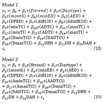
where the variables are as defined in Section 3.3 and et autocorrelated. In model 1 averaged temperature for each of the thermal regions considered, while in model 2 averaged temperature for coastal and inland as defined in Section 3.3.2 is used.
2.9 Model diagnostics and forecast accuracy measures
Diagnostic plots including information criteria will be used to assess the goodness of fit of the developed models. These are Akaike information criterion (AIC), corrected AIC (AICc), Bayesian information criterion (BIC), adjusted R squared (AdjR2) cross validation (CV), generalised cross validation (GCV), including deviance explained (DE). For assessing the quality of fit of the forecasted demand to the actual demand the root-mean square error (RMSE), mean-absolute error (MAE) and mean-absolute percentage error (MAPE) are used.
2.10 Forecast combinations
Literature has established that combining forecasts leads to more accurate forecasts (Bates and Granger, 1969; Devaine et al., 2012; Gaillard, 2015), including discussion on combining forecasts methods and development of some r statistical packages. Some of these r packages are 'forecastHybrid' (Shaub and Ellis, 2017) and 'opera' (Gaillard and Goude, 2016). The 'opera' r package was used in this study.
Let ytbe electricity demand at hour 20:00 as discussed in Section 2.4 and let there be Κ methods used to predict the next observations of yt, which shall be denoted by yt+1,yt+2,-, yt+m. Using k = 1,Κ methods,  , where ω Μ is weight.the combined forecasts will be given by
3. Results and discussion
3.1 Exploratory data analysis
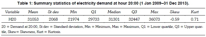
Table 1 presents a summary of statistics of electricity demand at hour 20:00 for the period 1 January 2009-31 December 2013. Minimum demand was 21 974 MW on Friday 25 December 2009, which was a summer day and maximum demand was 36 073 MW on Tuesday 13 July 2010, which was a winter day. The skewness and kurtosis presented in Table 1 show that the demand of electricity at 20:00 is non-normal. The mean and the median are not equal, which confirms that the distribution of electricity demand is not normally distributed. This is consistent with the density plot in Figure 1(b) where the bulk of the demand is to the left of the median demand of 31301MW.
A plot of electricity demand at 20:00hrs, together with the density plot, normal QQ-plot and the box plot, is given in Figure 1. Figure 1(a) shows that there is a slight upward trend between 2009 and 2010, followed by a downward trend from 2011 to 2013. The decrease in demand can possibly be attributed to the integration and use of renewable energy sources, as well as the positive effects of demand-side management.
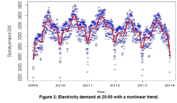
Figure 2 shows a plot of electricity demand with a fitted cubic smoothing spline as a nonlinear trend. The fitted values were extracted and used as input values for the variable 'fitrend' as discussed in Section 3.3.3.
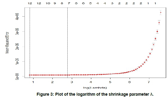
A plot of the logarithm of the shrinkage parameter λ given in Equation 6 is illustrated by Figure 3, where the dotted red line illustrates the cross-validation curve. The two dotted vertical lines illustrate two λ values: the one to the far left gives the minimum mean square cross-validated error, the other is such that it is within one standard error of the minimum (Hastie and Qian, 2016). The lambda to the left was found to be 0.79171 while the one to the right was found to be 2.84214.
A plot of the smoothed Daytype variable in Figure 4(a) shows that demand for electricity decreases during the weekend. Figure 4(b) shows the plot of the smoothed monthly variable and that demand for electricity increases significantly during the winter in South Africa compared with the non-winter periods. This was consistent with the results of modelling electricity demand in South Africa reported by Chikobvu and Sigauke (2013).
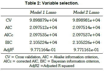
Selection of variables of the models given in Equations 18 and 20 was done using Lasso, as discussed in Section 2.2. Based on these criteria, CV, AIC, AICc, BIC and AdjR2, Model 1 Lasso in Table 2 was a better model and therefore selected. Model 1 was subsequently used for forecasting.
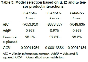
Model 1 in Equation 18 was then split into model without tensor interactions, called GAM-Lasso model, and model with tensor interactions. Models with tensor interactions gave GAM-ti-Lasso, GAM-te-Lasso and GAM-t2-Lasso, based on the tensor interaction r functions in 'mgcv' r package developed by Wood (2017) and as defined in Section 2.3. Tensor product interactions given by Equations 8 and 9 were compared and a better fit was found to be suitable for the two-way interactions, i.e., from Equation 8. Increasing the order of interactions as in Equation 9 gave a poor fit. The selection of the best model was based on the AIC, adjusted R squared, deviance explained, GCV, as well as on the amount of autocorrelation left in the residuals. Based on these models, GAM- -Lasso model was found to be the best model. A summary of these models is given in Table 3.
The fitted GAM-Lasso model was followed by tests for autocorrelations in the residuals, as shown in Figure 5.
A formal test using the Ljung-Box test gave a p-value of 2.2 X 10⁻¹⁶, which corroborated the auto-correlated residuals. Residuals of the GAM-Lasso model were then extracted to fit a SARIMA model.
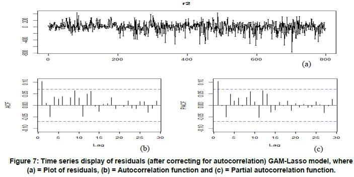
The best fitting model was found to be SARIMA(5,0,5) x (1,0,3) [7]. Residuals of this SARIMA model were then tested for autocorrelation, where the p-value of the Ljung-Box test was found to be 0.8658, implying that the residuals were not autocorrelated. Fitted values of the SARIMA model were extracted and subtracted from the data at 20:00hrs to get a new set of values for the response variable. This iterative process was followed as discussed in Section 3 and to refit the GAM-Lasso model. The diagnostic plots given in Figure 6 show that the GAM-Lasso model was a good fit to the data. Figure 6(c) shows that the distribution of the residuals was skewed to the left, while Figure 6(b) shows the residuals are clustered around zero, thus indicating their independence. A plot of the response variable versus the fitted values in Figure 6(d) shows a good fit. Figure 7 shows a time series display of residuals after correcting for autocorrelation.
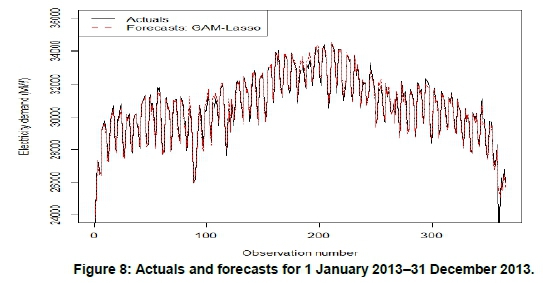
A formal test of the autocorrelation in the residuals using the Ljung-Box test was carried out and the p-value found to be 0.5496, implying that the residuals are not autocorrelated at the five percent level of significance. The model was then used for forecasting. Figure 8 shows agreement between electricity demand (solid black line) and forecasts (dashed red line) for 1 January 2013-31 December 2013.
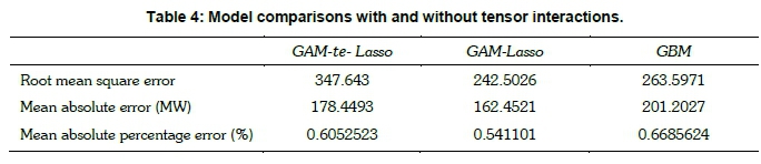
The SARIMA(3,0,7)x(1,0,1)[7] model was found to be the best fitting model after several attempts with SARIMA models. The procedure discussed in Section 4 was then carried out. A test of the residuals for autocorrelation yielded a p-value of 0.0151. Whilst most of the serial autocorrelation was removed, there was some autocorrelation left in the residuals. Diagnostic plots of the residuals, including the autocorrelation function and partial autocorrelation function, are given in the supplementary mate-rial.1 Model comparison of GAM-te-Lasso with GAM-Lasso and the gradient-boosting model was carried out. Based on the RMSE, MAE and MAPE, the GAM-Lasso was the best fitting model, followed by GAM-te-Lasso. Both methods outperformed the benchmark model - the gradient-boosting model.
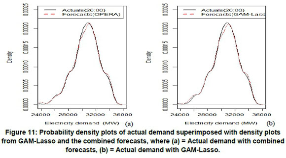
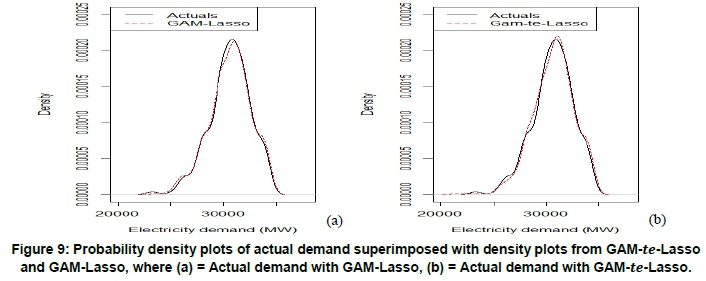
Figure 9 shows that the density plot of the forecasts from GAM-Lasso was a better fit to the density of the actual demand than the density plot of GAM-te-Lasso. Density forecasts are useful to decision-makers in power utility companies such as Eskom as they help to evaluate and hedge the financial risk accrued by demand variability and forecasting uncertainty (Hyndman and Fan, 2010).
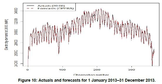
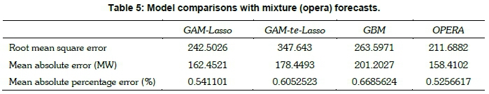
The 'opera' r package was used to combine the forecasts from GAM-Lasso, GAM-te-Lasso and gradient-boosting models. Based on the pinball loss function, the weights assigned to the forecasts from these three methods were respectively 0.648, 0.318 and 0.0337.
Table 5 indicates that the combined forecasts were more accurate compared with individual forecasts of the separate models, while Figure 10 shows that the forecasts from the combined models were in good agreement with the actual demand data.
The density plot of the combined forecasts in Figure 11 shows a better fit than that in the GAM-Lasso model.
4. Conclusions
An application of generalised additive models (GAMs) to medium-term forecasting of electricity demand using South African data was presented. Models were developed based on national aggregated average temperature and hourly electricity data from Eskom, South Africa's power utility. A comparative analysis was then done using a gradient boosting model. The forecasts from the three models were combined using a forecast combination algorithm where the average loss suffered by the models is based on the pinball loss function. This resulted in an improvement of the forecasts. The GAM-Lasso model gave more accurate forecasts compared with the GAM-Lasso model with tensor interactions. It was found that the probability density of the forecasts from the GAM-Lasso model and the combined forecast yielded a good fit to the density of electricity demand, compared with the density of
the forecasts from the GAM-te-Lasso. A major contribution of this paper is the inclusion of a nonlinear trend. Another contribution is the inclusion of temperature based on two thermal regions of South Africa. This study could be useful to system operators, including decision-makers in power utility companies such as Eskom for medium-term risk assessment and planning for maintenance scheduling of power plants.
Note
1. Supplementary data material with derivations and some of the tables and plots can be found at http://journals.assaf.org.za/jesa/rl/suppFiles/2428/0.
Acknowledgements
The author acknowledges the National Research Foundation of South Africa (Grant No: 93613) for funding this research and Eskom for providing the data.
References
Bates, J.M. and Granger, C.W.J. The combination of forecasts. Operational Research, 1969, 20(4): 451-468. [ Links ]
Bien, J., Taylor, J. and Tibshirani, R. A Lasso for hierarchical interactions. Annals of Statistics, 2013, 41(3): 1111-1141. [ Links ]
Chikobvu, D. and Sigauke, C. Modelling influence of temperature on daily peak electricity demand in South Africa. Journal of Energy in Southern Africa, 2013, 24(4): 63-70. [ Links ]
Clemen, R.T. Combining forecasts: A review and annotated bibliography. International Journal of Forecasting, 1989, 5: 559-583. [ Links ]
Debba, P., Koen, R., Holloway, J.P., Magadla, T., Rasuba, M., Khuluse, S. and Elphinstone, C.D. 2010. Forecasts for electricity demand in South Africa (2010-2035) using the CSIR sectoral regression model. Available online at http://www.energy.gov.za/IRP/irp%20files/CSIR_model_IRP%20forecasts%202010_final_v2.pdf. [ Links ]
Devaine, M., Gaillard, P., Goude, Y. and Stoltz, G. Fore casting the electricity consumption by aggregating specialized experts: A review of sequential aggregation of specialized experts, with an application to Slovakian and French country-wide one-day-ahead (half-) hourly predictions. Machine Learning, 2012, 90: 231-260. [ Links ]
Fan, S. and Hyndman, R.J. Short-term load forecasting based on a semi-parametric additive model. IEEE Transactions on Power Systems, 2012, 27(1): 134-141. [ Links ]
Fasiolo, M., Goude, Y., Nedellec, R. and Wood, S. N. Fast calibrated additive quantile regression, 2017. Available online at https://arxiv.org/abs/1707.03307 (accessed 10 November 2017). [ Links ]
Friedman, J.H. Multivariate adaptive regression splines. The Annals of Statistics, 1991, 19(1): 1-141. [ Links ]
Friedman, J., Hastie, T., Simon, N. and Tibshirani, R. Lasso and elastic-net regularized generalized linear models: glmnet r package version 2.0-10, 2017. Available online at https://cran.r-project.org/web/packages/glmnet/glmnet.pdf (Accessed on 7 May March 2017). [ Links ]
Gaillard, P. Contributions to online robust aggregation: Work on the approximation error and on probabilistic forecasting. PhD Thesis, 2015, University Paris Sud, France. [ Links ]
Gaillard, P., Goude, Y. and Nedellec, R. Additive models and robust aggregation for GEFcom2014 probabilistic electric load and electricity price forecasting. International Journal of forecasting, 2016, 32: 1038-1050. [ Links ]
Goude, Y., Nedellec, R. and Kong, N. Local short and middle term electricity load forecasting with semi-parametric additive models. IEEE Transactions on Smart Grid, 2014, 5(1):440- 446. [ Links ]
Hastie T. and Tibshirani, R. Generalized additive models (with discussion). Statistical Science, 1986, 1: 297-318. [ Links ]
Hastie, T. and Tibshirani, R. Generalized additive models, 1990, Chapman & Hall. [ Links ]
Hong T. and Fan S. Probabilistic electric load forecasting: A tutorial review. International Journal of Forecasting, 2016, 32: 914-938. [ Links ]
Hong, T., Pinson, P., Fan, S., Zareipour, H., Troccoli, A. and Hyndman, R.J. Probabilistic energy forecasting: Global Energy Forecasting Competition 2014 and beyond. International Journal of Forecasting, 2016; 32(3): 896-913. [ Links ]
Hyndman, R.J. and Fan, S. Density forecasting for long- term peak electricity demand, IEEE Transactions on Power Systems, 2010, 25(2): 1142-1153. [ Links ]
Hyndman, R.J. and Athanasopoulos, G. Forecasting: principles and practice, 2013. Available online at https://www.otexts.org/fpp/9/1 (accessed 26 March 2017). [ Links ]
Hyndman, R.J. forecast: Forecasting functions for time series and linear models. R package version 8.1, 2017. Available online at http://github.com/robjhynd-man/forecast. [ Links ]
Laurinec P. Doing magic and analyzing seasonal time series with GAM (Generalized Additive Model) in R, 2017. Available online at https://petolau.github.io/Analyzing-double-seasonal-time-series-with-GAM-in-R/_(accessed 23 February 2017). [ Links ]
Meier, L., van de Geer, S. and Bühlman, P. The group lasso for logistic regression. Journal of the Royal Statistical Society B, 2008, 70(1): 53-71. [ Links ]
Munoz, A., Sanchez-Ubeda, E.F., Cruz, A. and Marin, J. Short-term forecasting in power systems: a guided tour. Energy Systems, 2010, 2: 129-160. [ Links ]
Pierrot, A. and Goude, Y. Short-term electricity load forecasting with generalized additive models. Proceedings of ISAP Power, 2011: 593-600. [ Links ]
Sigauke, C. and Chikobvu, D. Short-term peak electricity demand in South Africa. African Journal of Business Management. 2012, 6(32): 9243-9249. [ Links ]
Sigauke, C., Verster, A. and Chikobvu, D. Extreme daily increases in peak electricity demand: Tail-quantile estimation. Energy Policy, 2013, 53: 90-96. [ Links ]
Shaub, D. and Ellis, P. Convenient functions for ensemble time series forecasts. R package version 1.1.9, 2017. Available online at https://cran.r-project.org/web/packages/forecastHybrid/forecastHybrid.pdf. [ Links ]
Simpson, G. Modelling seasonal data with GAMs, 2014. Available online at http://www.fromthebottomofthe-heap.net/2014/05/09/modelling-seasonal-data-with-gam/ (accessed 26 February 2017). [ Links ]
Takeda, H., Tamura, Y. and Sato, S. Using the ensemble Kalman filter for electricity load forecasting and analysis. Energy, 2016, 104: 184-198. [ Links ]
Tibshirani, R. Regression shrinkage and selection via lasso. Journal of the Royal Statistical Society. Series B (methodology), 1996, 58(1): 267-288. [ Links ]
Van Buuren, S. and Groothuis-Oudshoorn, K. MICE: Multivariate imputation by chained equations in R. Journal of Statistical Software, 2011, 45(3): 1-67. [ Links ]
Wheeler M.W. Bayesian additive adaptive basis tensor product models for modelling high dimensional surfaces: An application to high-throughput toxicity testing, 2017. Available online at https://arxiv.org/abs/1702.04775 (accessed 4 April 2017). [ Links ]
Wood, S. Generalized additive models: An introduction with R, 2006, London: Chapman and Hall. [ Links ]
Wood, S. MGCV rpackage, version 1.8-17, 2017. Available online at https://cran.r-project.org/web/pack-ages/mgcv/index.html (accessed 15 February 2017). [ Links ]
Wood, S. P-splines with derivative based penalties and tensor product smoothing of unevenly distributed data. Statistics and Computing, 2017, 27: 985-989. [ Links ]
Xie, J., Hong, T. and Kang, C. From high-resolution data to high-resolution probabilistic load forecasts. Transmission and Distribution Conference and Exposition,IEEE/PES, 2016 DOI: 10.1109/TDC.2016.7520073. [ Links ]
Yuan, M. and Lin, Y. Model selection and estimation in regression with grouped variables. Journal of Royal Statistical Society Series B, 2006, 68: 49-67. [ Links ]
Ziel, A. Modelling and forecasting electricity load using Lasso methods. Modern Electric Power Systems, 2016. DOI: 10.1109/MEPS.2015.7477217. [ Links ]
Ziel, F. and Liu B. Lasso estimation for GEFCom2014 probabilistic electric load forecasting. International Journal of Forecasting, 2016, 32: 1029-1037. [ Links ]
Zou, H. and Hastie, T. Regularization and variable selection via the elastic net. Journal of the Royal Statistical Society. Series B (methodology), 2005, 67(2): 301-320. [ Links ]
Corresponding author: Tel: +27 15 962 8135; mail: caston.sigauke@univen.ac.za

