ARTICLES

 

Numerical optimisation of a small-scale wind turbine through the use of surrogate modelling

 

 

Gareth Erfort^*; Theodor Willem von Backstrom; Gerhard Venter

Department of Mechanical & Mechatronic Engineering, Stellenbosch University, Stellenbosch 7945, South Africa

 

 

---

ABSTRACT

Wind conditions in South Africa are suitable for small-scale wind turbines, with wind speeds below 7 m.s^-1. This investigation is about a methodology to optimise a full wind turbine using a surrogate model. A previously optimised turbine was further optimised over a range of wind speeds in terms of a new parameterisation methodology for the aerodynamic profile of the turbine blades, using non-uniform rational B-splines to encompass a wide range of possible shapes. The optimisation process used a genetic algorithm to evaluate an input vector of 61 variables, which fully described the geometry, wind conditions and rotational speed of the turbine. The optimal performance was assessed according to a weighted coefficient of power, which rated the turbine blade's ability to extract power from the available wind stream. This methodology was validated using XFOIL to assess the final solution. The results showed that the surrogate model was successful in providing an optimised solution and, with further refinement, could increase the coefficient of power obtained.

Keywords: optimisation; support vector regression; NURBs; C_p

---

 

 

1. Introduction

In a study by Cencelli [1], multi-objective optimisation was looked at for small wind turbines, typically operating at wind speeds below 7 m.s^-1. Cencelli initially optimised the aerodynamic performance of this turbine by selecting various standard wind turbine blade profiles, blending their geometries, and calculating the lift and drag coefficients of the blended profiles by means of the open access software XFOIL [2]. Wise [13] used a family of airfoils (NACA four digit series) for optimisation of a similar small turbine. As Wise limited the study to a single family or airfoils, Wessels [12] asked if the pre-selec-tion of foil profiles unnecessarily constrained the outcome and therefore sought to describe a general foil without referring to an existing foil type. Wessels compared the representation of airfoils by means of non-uniform rational B-splines (NURBs), describing either their camber and thickness distribution or the upper and lower surface XY co-ordinates to their standard definitions. Wessels was able to describe foils used by both Wise and Cencelli, and others, through NURBs. Cencelli and Wise made use of blade element momentum theory to model the wind turbine and gradient-based optimisation methods. The same turbine model was utilised, however, as the number of design variables significantly increased, various optimisation methods were examined. Cencelli and Wise provided a suitable baseline and allowed for a comparison of achieved optima. Cencelli optimised the foil at each station individually. Thereafter the combination of stations into a single blade was optimised for chord length and twist to obtain the best annual energy production (AEP) based on Cp values. This meant that five separate optimisation tasks had to be completed. Wise's approach was limited to a specific family of blades (NACA 4-digit) and combined the optimisation into one task. Wise also made use of a surrogate to describe the turbine system and changed the objective from the AEP to a non-weighted average of the blade C_pand used random starting points to alleviate the possibility of local minima, as a traditional gradient based approach would be more susceptible to these minima and required multiple random starting points. To build the surrogate model Wise used the support vector regression technique (SVR).

The aerodynamic design of a wind turbine for specific conditions is a complex problem with many design variables such as blade disc diameter, speed of rotation, blade section shape and wing planform shape [14]. Blade section shapes are often selected from existing standard families of blades. This investigation presents a method that determines original blade profiles during the optimisation process. The blade profile, camber line and thickness distributions were each described by NURBs.

The description of each blade profile requires 13 variables at each of the four design radii, excluding the variation in chord length and station orientation angle, leaving 15 variables per station. The optimisation adjusted these variables, resulting in new foil profiles, sizes and angles of attack at each station. Optimisation of such a system is challenging due to the large number of design variables. Each new profile must then be evaluated for lift and drag coefficients, Cl and Cd, which can be a time-intensive process. The blade element momentum theory, given the Cl and Cd at each blade section radius, allows for the calculation of characteristics of a full blade for a given flow condition. The power coefficient, C_p, of a turbine can be determined as well as its annual power production for a given wind velocity probability distribution over the period, given the Cl and Cd. In addition to this, optimisation techniques can be applied to find a combination of blade shape and turbine characteristics (rotational speed, blade length, blade twist and pitch angle.) that would result in the maximum average Cp. In this investigation a surrogate was created to provide the Cl and Cd for a wide range of foil shapes quickly, using SVR techniques based on coefficients obtained from an open source airfoil section performance prediction code[2].

 

2. Methodology

2.1 Blade element momentum theory

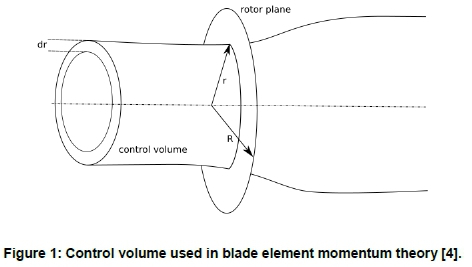
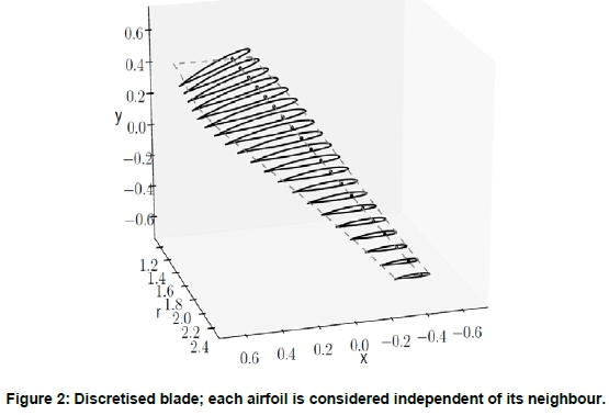
The blade element momentum theory partitions a rotating blade into 2D annular rings as shown in Figure 1. This theory builds on the actuator disk model described by Hansen [4] and assumes that there is no influence adjacent to the ring that affects the coefficients of lift or drag and, therefore, enables piece-wise analysis of a blade as discrete airfoil sections, as shown in Figure 2. The blade element momentum examines the flow around a foil using the momentum equation and derives equations for the forces acting on the blade. It also describes induction factors, variables used to account for changes in both the axial (a) and angular momentum (α'), as the flow moves through the blade disc. The forces on the blade are expressed in terms of the known flow conditions and the induction factors, as yet unknown. An iterative process is preformed to calculate these induction factors in order to balance the Bernoulli equation before and after the disk. Furthermore, there are adjustment factors that are used to determine the induction factors. The Prandtl's tip loss factor is used to correct the assumption of infinite blades and Glauert's correction factor is used to ensure the axial momentum factor does not violate the simple momentum theory. This process is described in full in Hansen [4]. The algorithm used to calculate the blade performance is described in Table 1.

 

 

 

 

Assuming there is a linear variation in each radial station (r), the tangential load between these points can be estimated according to Equation 1.

where i is the current position and A_i, B_iare defined according to Equation 2.

This in turn allows a definition of the torque contribution for each portion between r_iand r_i+1as in Equation 3.

The total torque is then worked out by multiplying the cumulative contribution of Equation 3 by the number of blades given by Equation 4.

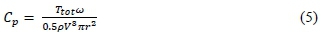
The torque is then used to determine how much power is produced for the given regime, followed by normalisation to give a non-dimensionalised co-efficient of power according to Equation 5.

2.2 Optimisation

This investigation took a step further than Wise [13], with the blade profiles not limited to a specific family or combination of families. Instead by using a NURB description of a foil, as detailed by Wessels [12], the shape had more scope for variation. The optimisation problem is stated as in Equation 6.

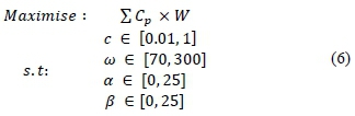
A Weibull weighting function (W) based on wind speed was applied to the Cp values, and the summation was then set as the objective function. The Cp function value was based on blade shape (as defined by Equations 8-10 in Section 2.4), flow regime and angle of attack, resulting in an input vector of 61 variables for simultaneous optimisation. The constraints in this optimisation related to chord length (c), rotational speed (ω), angle of attack (α) and twist (β) in the blade. The starting population for optimisation included the final solution of Wise, in the form of the seed vector. A genetic algorithm was used to do the optimisation in order to reduce the effect of local minima and better sampling of the large domain.

2.3 Genetic algorithm

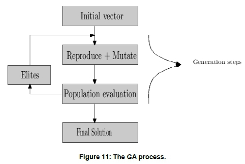
The optimisation is performed with a genetic breeder algorithm. The algorithm requires an objective function, the upper and lower limits of all the parameters within the objective function and an initial population. In this investigation a starting vector was used to create a population of equally sized vectors. These vectors were random 'mutations' of the original, with the degree of variation also being a value the user could set. The original population included the initial seed vector. The population spread increased with the magnitude of mutation allowing for a greater variation of test vectors. The next generation was obtained by selecting a percentage of the best performing members of the population and breeding them. The threshold controlling the percentage of members selected for breeding was a user defined variable. In addition there were 'elite' members of each generation, which were guaranteed a place in the future generation. Once the solution improvements between generations was within tolerance, the best performing vector of the last generation was returned as the optimised result [9].

In this investigation a population size of 50 was set per generation. A threshold for breeding selection was set at 15% and the four best performing vectors formed the elite sample set. After testing various algorithm settings, it was found that a mutation factor of 0.2 with a total of 12 generations provided the best results.

2.4 Non uniform rational B-splines

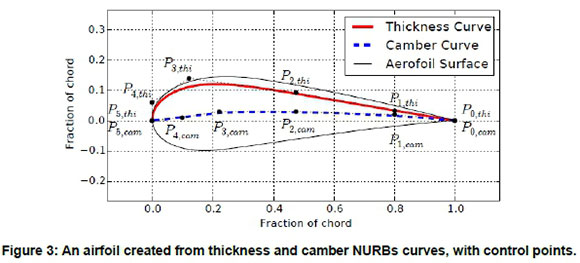
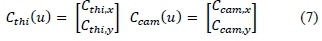
The NURBs configurations are able to accurately and reliably represent the shape of an airfoil. These configurations describe a complex curve through a few x, y coordinates, subsequently lending themselves to optimisation, with minor adjustments resulting in a wide range of curves. A full description of NURBs is given by Wessels [12], while also describing the methodology for creating airfoils. The adopted methodology was the thickness-camber approach, where two NURBs were used to describe the thickness and camber curves respectively much like the NACA four digit scheme; the results of this NURB description are shown in Figure 3. This foil was built by defining the thickness curve (C_thi(u)) and a camber (C_cam(u)) curve according to Equation 7, for a non-periodic knot vector (u) between 1 and 0, a point on each curve is found in terms of the x y coordinate system.

 

 

The upper and lower surfaces were, thus, created by adding/subtracting the y-coordinate of the thickness curves perpendicularly from the camber curve, expressed as Equation 8.

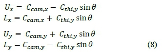
where the angle θ is the inclination of the camber curve, which was found using a central finite difference method and calculated with Equation 9.

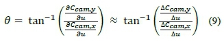
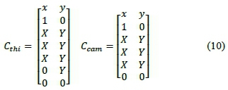
The trailing edge and leading edge had fixed coordinates to also control the ambiguity associated with angle of attack when describing a foil through NURBs. This meant the number of control points (x and y coordinates) to describe each of the thickness and camber curves were six and five respectively, but the total number of variables amounted to only 13. The reduced number of variables required is attributed to fixed leading and trailing edges. In the C_thimatrix points 0 and 5 are fixed in space and the x coordinate of point 4 is set to 0. In the Ccam points 0 and 4 are also fixed, as shown in Equation 10.

2.5 Surrogates

Surrogates are simplified mathematical models of a more complex system. These models reduce time in calculations, remove numerical noise and make it easier to solve larger problems by reducing the coupling of complex interactions to single functions. In particular the use of such a model for this problem drastically reduces the run-time during optimisation. As the optimisation process calls for a model evaluation many times while finding the optimum, surrogate models were used to provide a fast response. SVR appeared to be robust and achieved good accuracy through the availability of parameters that could be fine-tuned [5, 6]. To build the SVR surrogate, the model needs to be trained and adjusted accordingly based on a testing set. The training and testing data sets can be one large set or two distinct sets. The latter is preferred, in that there is no bias on the model score when evaluating the test data.

The workspace for the foil involved 13 control points, as outlined in Equation 10, an angle of attack and a Reynolds number, resulting in a 15-variable surrogate model. Data sets for training were created in XFOIL using the latin hypercube sampling technique and the testing data was generated in the same program but through randomised selection. In doing so the training set was ensured to more effectively sample the workspace [7], while the test set may have overlaps but provides a suitable selection for the testing criteria.

XFOIL is an open source package that uses the panel method and boundary layer calculations on the blade surface to determine coefficients of lift and drag for a prescribed airfoil. The package requires a foil definition in the form of a text file, angle of attack and flow conditions. The run-time of XFOIL is not fixed but the user can limit the number of iterations to perform. If the program fails to converge before the maximum iterations are reached it will not provide any data for analysis. The result of XFOIL is a table listing the angle of attack and corresponding Cl and Cd values. The program is, however, not very robust and has a tendency to hang or crash. The possibility of hanging or failure meant the program was not suitable for direct use in optimisation. A control program written in Python [3] uses the latin hypercube sampling to select data points for testing and training. The number of points in each set is controlled by the user and listed in an array. The array is cycled through a multi-threading module. The multi-threading is done to save time and also as a safeguard against the XFOIL program: should it hang while evaluating a data point, another thread can continue down the array. The second safeguard against XFOIL crashing was to handle it in a robust manner. If the user prescribed an angle of attack the program would be instructed to test a sequence of a's, and output the result. This approach assumes that XFOIL may fail at or near the desired α, but it would not fail at all locations near the point of interest. Based on the output, a line can be extrapolated through the data points and the angle of attack in question can be interpolated.

The Scikit-learn module [8] is used to build the SVR models. This module allows for a choice of kernel and its related build parameters (kernel degree, epsilon tube, penalty factor, etc). The SVR can be expressed as Equation 11.

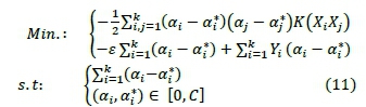
where the C is the penalty factor and k(x_i, X_j) is the kernel function. Within the SVR module the radial basis function kernel is chosen. Initial testing shows it to have a better score (R²), a valuation of how good the regression performed, than for example a polynomial kernel. It was found that the surrogate was most responsive to the penalty factor and the kernel coefficient γ as used in the radial basis function kernel given by Equation 12.

These two parameters were then evaluated through a multi-grid analysis which ran through numerous combinations of C and γ while trying to improve the score. The score of the surrogate, also known as the coefficient of determination (R²), is a measure of variance between model predictions and test set targets. The training data set is used during the grid analysis and a separate test data set created in XFOIL is then used to evaluate the grid refined surrogate.

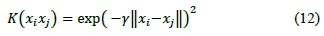
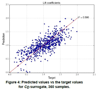
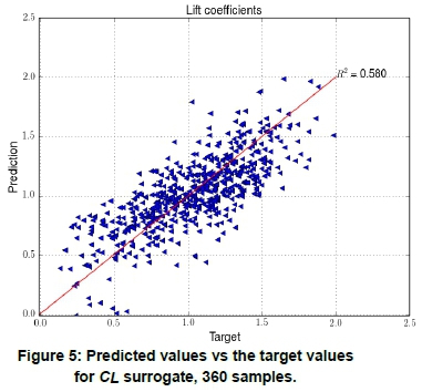
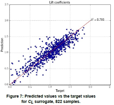
The oversight program implemented in Python allows for the development of various size data sets in a relatively short time. The latin hypercube sampling prescribed data set was 900 samples in size and 90% of those points were successfully evaluated through XFOIL. The built-in libraries in Python did not handle data sets larger than this, effectively setting the ceiling on data set size. Figures 4 and 5 show an example of surrogate scores based on a sample set of 360 points, the red line indicating where the predicted values and target values are to meet. Due to the size of the data sets the scores are relatively low, and we have noticeable scatter on Figure 5. When comparing these to Figures 6 and 7, which are based on a sample set of 822 points, there is improvement in the scores, with the prediction points tighter along the line.

 

 

 

 

 

 

 

 

2.6 Using the NURBs to build surrogates

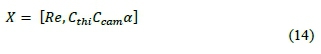
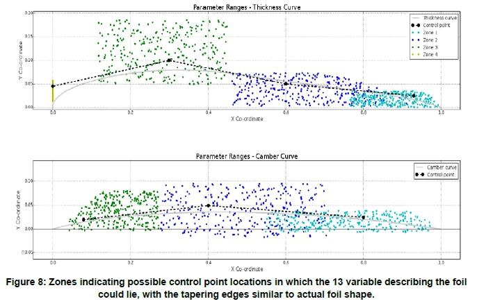
Each foil is described by 13 variables. The upper and lower limits of these variables have been determined above and are used to define the solution space. Figure 8 shows the solution space of the thickness and camber curves in terms of their possible [X, Y] coordinates, as illustrated in Equation 10. Each control point is allowed to be within zones depicted. This figure also illustrates by way of example how the control points affect thickness and camber curves. The thickness curve has seven variables, the x position of the nose being fixed, and the camber curve has six variables. The limits for viable co-ordinates were defined as a selectable attribute in Python. The solution space shown approximates the shape associated with a foil with tapering edges. Equation 14 shows the form of the input vector to the surrogate. It comprises the Reynolds number (Re), the X and Y coordinates for the thickness and camber curves as stated in Equation 10, and the angle of attack (α).

2.7 Multiple preference points method

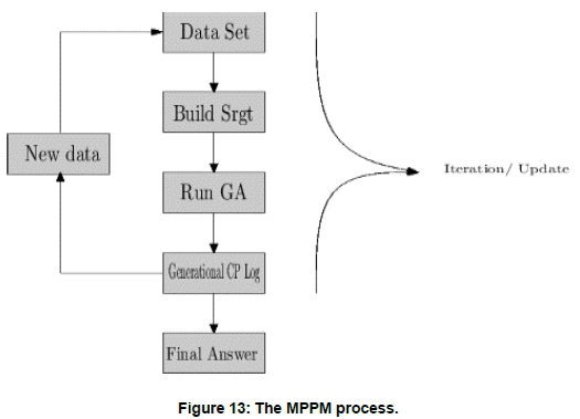
As stated earlier, the surrogate models' prediction is heavily based on the number of sample points. Generating these sample points can take time, especially if utilising the optimum latin hypercube method. A structured latin hypercube tries to achieve the same effectiveness while reducing the computational time [13]. The problem is one of effectively sampling the entire range of possible solutions. If there is a weak area of prediction where the surrogate may give incorrect or highly optimistic results, the optimiser would exploit this. A way to counteract this effect is to sample in the areas where the optimiser will drive the solution. As this information is not available beforehand, the MPPM approach is used to increase the sample size while optimising. This method of surrogate building, along with others, is described in Shao [10].

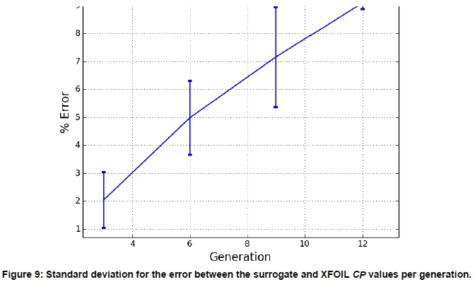
Initially, a small sample set of 300 is used to build the surrogate model and then run through the genetic algorithm. The genetic algorithm (GA) runs for 12 generations, due to the percentage error reaching the maximum allowable value of no more than 10% (see Figure 9), and at the end of each generation the best performing vector is logged along with its Cp value. This log is used to identify any large changes in C_p, enabling identification of significantly different solution vectors which are then added to the initial training set. One run through the GA constitutes a single iteration, at the end of which the surrogate is updated. This inherently random, yet evolutionary, system means there is no set number of points added to the training set at each update. The most significant changes usually occur early in the optimisation and after a certain generation the error became too large. Testing revealed a suitable cut-off in terms of how many generations the GA has to run.

 

3. Results

The surrogate based on 822 points was run once through the GA. It was capable of predicting reasonable Cl and Cd values but, as seen in Figures 6 and 7, there was still scatter in both models. The surrogate was tested against XFOIL for various cases and its accuracy was not sufficient. Thus, when run through the optimiser the improvements seen were, in fact, not real. The surrogate ventures into territory not sufficiently sampled initially. Any ill-defined region within the surrogate model will be exploited by the optimiser during run time. The history plot of the optimiser is seen in Figure 10. Key points are then run through XFOIL and plotted on the same graph. This highlights the inaccuracies in using this surrogate.

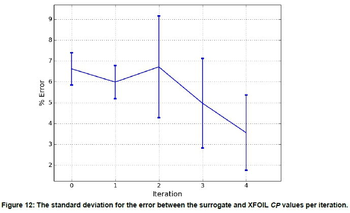
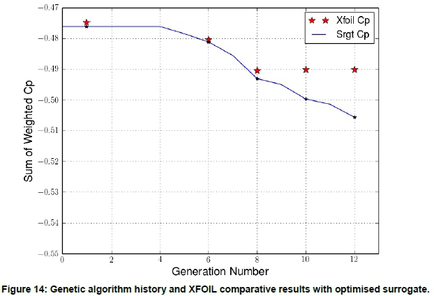
The single-build approach was not effective, so MPPM was adopted. When using the GA, the majority of the new data points were from early generations. Figure 10 highlights the increasing discrepancy between surrogate and XFOIL after successive generations, and Figure 11 shows the flow diagram for the GA sequence. For the MPPM method the generational limit was set at 12. This was after testing found the average error was approximately 9% in this generation. Figure 12 shows the decrease in an average error from 6.6% to 3.5%, through using MPPM (flow diagram seen in Figure 13). The results presented in Figure 14 are for a surrogate with 1088 samples. While the overall error is reduced, the deviation has increased. The MPPM approach is utilised to minimise the error but there is a cumulative affect still present. This is assumed to be the cause of the deviation seen in Figure 12. Figure 14 shows the XFOIL and updated surrogate data to be more closely aligned. This validated the MPPM approach and allowed confidence to be expressed in the surrogate predictions.

 

 

 

 

3.2 Final result

Figure 15 shows the starting Cp curves, from the solution presented by Wise [13], and the final Cp curves after optimisation. The curves show the C_pas reported from both XFOIL and the iteratively updated surrogate model. Wise's final solution was a blade optimised to work between 5 and 6 m.s^-1 while, in comparison, this solution was over a larger wind speed range. Over the 5-6 m.s^-1 range Wise has a higher Cp with a drop after 6 m.s^-1. The final Cp curve is consistent over the entire range of wind speeds. The optimiser increased the higher wind Cp while lowering the peak achievable C_p.

 

 

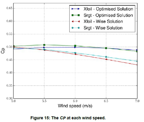
Figure 16 shows the optimised blade shape overlaid on the original shaped specified by Wise. Noticeable differences include a longer foil at the hub (Fig 16a), a narrower tail in the mid-section (Fig 16b), and a more cambered tip (Fig 16d).

 

4. Conclusions

This paper sought to optimise the aerodynamic design of a small wind turbine. The methodology was based on the use of a surrogate model, which incorporated both the geometric constraints of the blade and the turbines operation conditions. Surrogate models have been shown as effective tools when coupled with optimisation algorithms. The comparison of the final result with XFOIL meant the solution had to be run while getting lift and drag variables from XFOIL. This process highlighted the surrogate's time gains, as the model took approximately 36 minutes to run with XFOIL but less than one minute using the surrogate. The quality of the surrogate greatly affects the outcome, and care must be taken in how it is built. Attention must be given to the training and testing data set, ensuring that it sufficiently samples the design space. The iterative approach of MPPM proved successful in reducing surrogate error with minimal additional data points. However, the approach taken to identify the most preferred points should be adjusted, as it did not take sufficient data near the end of each optimisation run. Based on these results it can be assumed that additional iterative updates to the surrogate through MPPM would improve its accuracy. The limitation in this project was the use of built-in Python libraries. The Python library began hanging once training sets exceeded 900 points. A customised library could overcome this and allow for several updates on the surrogate. Overall, the methodology to wind turbine optimisation has proven effective, as it improved on a previously optimised solution.

 

References

[1] Cencelli, N.A. Aerodynamic optimisation of a small-scale wind turbine blade for low windspeed conditions. 2006. Masters thesis, University of Stel-lenbosch, Stellenbosch, South Africa.         [ Links ]

[2] Drela, M. 2001. Xfoil 6.94 user guide. Aeronautics, and Astronautics Engineering, Massachusetts Institute of Technology, Cambridge, MA, USA.         [ Links ]

[3] Hansen, M.O.L. 2008. Aerodynamics of wind turbines. Earthscan.         [ Links ]

[4] Ju, Y., Zhang, C. and Ma, L. 2016. Artificial intelligence metamodel comparison and application to wind turbine airfoil uncertainty analysis. Advances in Mechanical Engineering, 8(5).         [ Links ]

[5] Li, Y.F, Ng, S.H., Xie, M. and Goh, T.N. 2010. A systematic comparison of metamodeling techniques for simulation optimization in decision support systems. Applied Soft Computing 10(4): 1257-1273.         [ Links ]

[6] Mckay, M.D., Beckman, R.J. and Conover, W.J. 2000. A comparison of three methods for selecting values of input variables in the analysis of output from a computer code. Technometrics, 42(1): 5561.         [ Links ]

[7] Pedregosa, F., Varoquaux, G., Gramfort, A., Michel, V., Thirion, B., Grisel, O., Blondel, M., Prettenhofer, P., Weiss, R., Dubourg, V. and Vanderplas, J. 2011. Scikit-learn: Machine learning in Python. Journal of Machine Learning Research 12(Oct), 2825-2830.         [ Links ]

[8] Python Software Foundation. Python language reference, version 2.7.         [ Links ]

[9] Salomon, R. 1998. Evolutionary algorithms and gradient search: similarities and differences. IEEE Transactions on Evolutionary Computation 2(2): 45-55.         [ Links ]

[10] Hao, T. and Krishnamurty, S. 2007. A hybrid method for surrogate model updating in engineering design optimization. ASME. International Design Engineering Technical Conferences and Computers and Information in Engineering Conference, Volume 6: 33rd Design Automation Conference, Parts A and B:345-370.         [ Links ]

[11] Smola, A.J. and Schólkopf, B. 2004. A tutorial on support vector regression. Statistics and computing 14(3): 199-222.         [ Links ]

[12] Wessels, F.J.L., Venter, G. and Backstrom, T.W. 2012. An efficient scheme for describing airfoils using non-uniform rational b-splines. ASME. Turbo Expo: Power for Land, Sea, and Air, Volume 6: Oil and Gas Applications; Concentrating Solar Power Plants; Steam Turbines; Wind Energy ():969-977.         [ Links ]

[13] Wise, J. 2008. Optimization of a low speed wind turbine using support vector regression. Masters thesis, Stellenbosch University, Stellenbosch, South Africa.         [ Links ]

[14] Zhang, Z. 2012. Performance optimization of wind turbines. PhD thesis, University of Iowa, Iowa, USA.         [ Links ]

 

 

* Corresponding author: Tel: +27 21 808 4264; email: erfort@sun.ac.za