ARTICLES

 

Characterisation of wind speed series and power in Durban

 

 

Ayele Nigussie Legesse^*; Akshay Kumar Saha; Rudiren Pillay Carpanen

Discipline of Electrical, Electronic and Computer Engineering, School of Engineering, University of KwaZulu-Natal, Durban 4041, South Africa

 

 

---

ABSTRACT

Both the planning and operating of a wind farm demand an appropriate wind speed model of its location. The model also helps predict the dynamic behaviour of wind turbines and wind power potential in the location. This study characterises the wind speed series and power in Durban (29.9560°S, 30.9730Έ), South Africa, using Markov chain and Weibull distribution. Comparison of statistical quantities of measured and Markov model-generated wind speed series revealed that the model accurately represented the measured wind speed series. The Markov model and Weibull distribution were also compared through their corresponding probability density functions. The root mean square error of the Markov model against the measured wind speed series was nearly one-tenth that of the Weibull distribution, indicating the effectiveness of the former. Finally, the analysis of wind power density showed that Durban and its environs need large wind turbines with hub heights greater than 85 m for efficient utilisation of the available wind energy.
Highlights:
• Wind speed series in Durban can be characterised using the Markov chain model, and the corresponding power can be fairly predicted using the model.
• Compared to the conventional Weibull distribution, the Markov chain model accurately represents the wind speed series in Durban.
• Durban and its environs require wind turbines with heights higher than 85 m for efficient operation.

Keywords: dynamic simulation, Markov chain, Weibull distribution, wind turbine

---

 

 

1. Introduction

Depletion of fossil fuel reserves, global warming, security concerns, and rising commodity prices are pushing the world to go green. Much attention is currently given to the development of renewable energy, among which harnessing wind energy is the cheapest alternative[1-3]. Feasibility studies related to wind power require an appropriate wind speed model of a site [4, 5]. These models are also important in planning and operating wind turbines. Hence, the wind speeds of a specified site should be appropriately characterised to determine wind energy potential and attain comprehensive results in the investigations of the dynamics of the wind turbines [4, 6, 7]. Moreover, a good characterisation of wind speed helps transmission system operators in scheduling their power dispatch [4].

Wind is a random stochastic process whose dynamic behaviour can be represented by a stochastic model [8]. Naturally, it depends on pressure gradient, waves, jet streams, and local weather conditions [9]. Its stochastic modelling is a complicated task because of its strong variability in time and land terrains. Over a year, wind speed is periodic, showing seasonal variations; however, hourly average wind speed is a stochastic process with a Weibull probability density function; whereas within minutes, it follows a Gaussian distribution [10].

Different methods have been employed for time series characterisation of wind processes. Traditionally Weibull distribution is widely used to represent wind speed series at a given site [4, 11-13]. Normal, Gamma, Lognormal or combination of these distributions with Weibull distribution [4, 7, 14- 16], empirical wavelet [17] or Kernel density method [18] can also be used to model wind speed series. Shokrzadeh et al. [19] and Kazemi and Goudarzi [20] employed advanced parametric and nonparametric and least square approximation methods to forecast wind power. A typical distribution may not necessarily represent the cumulative wind behaviour of all locations in a region [7]. Thus, the wind speed for a particular location needs to be modelled. The above distributions cannot be used, however, when chronology is considered [4]. A rough observation on the raw wind speed data from Durban demonstrated that the current wind speed depended on the previous wind speed, indicating that chronology should be considered in modelling the wind speeds. Evolutionary algorithms such as genetic algorithm and local search technique are also used in wind speed modelling [21] despite their time consuming procedure [4].

The Markov chain model, which retains chronology and consumes less time, could, therefore, be employed to synthesise wind speed time series for dynamic simulation and wind power forecasting[10, 22-24]. The accuracy of a Markov model increases with its order [22]. The first-order model is often adopted for its simplicity and economic computing time [24]. A modified Markov model may show better performances than the corresponding normal model in preserving the properties of wind speed se-ries[25]. Particularly, the second order semi-Markov process is more suitable for processes characterised by states with variable durations [10].

Few efforts have been made to characterise wind speeds and power for electric generation in South Africa using computer algorithms and frequency distribution methods [26-28]; however, the Markov model has never been used for characterising wind speed series in Durban. As wind speed models strongly depend on location, an investigation into the wind speed series at the site is vital. This study, therefore, used the first order Markov chain model to characterise the wind speed series in Durban using fixed-step duration between states. The model was also compared with Weibull distribution. The comparison showed that the Markov model was more effective than Weibull distribution. Finally, Weibull and Gaussian probability density functions, along with the Markov model, were employed to produce synthetic wind speed series over minute and second intervals respectively. Generation of artificial wind speed series was crucial for the dynamic simulation of wind turbines.

 

2. Data preparation and analysis

2.1 Wind speed data

The data used in this investigation was obtained from South African Weather Services. Hourly wind speed measurements were taken at Durban South Merebank (DSM) (29.9560°S, 30.9730°E) from January 2014 to December 2015. Anemometers were installed at the station at 8 m hub height to measure wind speed from the DSM weather station, notwithstanding the height of the tower of a wind turbine that exceeded 8 m.

2.2 Data analysis

These wind speed data are converted to the corresponding higher hub height data by the power law wind speed profile [29] defined by Equation 1. Wind speed directions were not considered in this investigation as wind energy density mainly depends on the speed.

where

v_h2=wind speed at hub height 2;

v_h1= wind speed at hub height 1;

h₂= hub height 1;

h₁= hub height 2;

a = Hellman Exponent.

Figure 1 shows a two year distribution of wind speed series at DSM at 70 m hub height. These hourly values are statistically analysed to generate monthly hourly wind speed values, subsequently used to sketch the wind speed contour maps for Durban. Figures 2 and 3 show the wind speed contour maps at 8 m and 70 m hub heights at the DSM weather station respectively. The hourly wind speed values shown in Table 1 were obtained at an altitude of 70 m and range from 0 to 23 m/s. Average monthly hourly wind speeds, however, ranged from 1.5 to 12 m/s. The wind speed, which is very stochastic, highly depended on temperature variations as shown in Figure 2, a contour map for hourly monthly wind speeds. Wind being created by differential heating of the earth's surface by the sun, it increased with solar radiation.. The daily maximum wind speed was observed from 13h00 to 16h00 where the temperature was also maximum, whereas, the minimum speed occurred after midnight. Wind speed density was high during working hours, which is vital for wind turbine operators. Furthermore, Figure 2 shows the dependence of wind speed on seasonal variations. From December to March, relatively hot months, the wind speeds were relatively high (2.5 - 5.5 m/s monthly average wind speed). On the other hand, from April to August, usually corresponding to the dry season, low wind speeds (1.5-3 m/s monthly average wind speed) were expected. September, October and November saw monthly average wind speeds ranging from 24.5 m/s. Wind speed also increased with hub height, as shown in Figure 4.

 

 

 

 

 

 

3. Methods, results and discussion

3.1 Markov chain model

The Markov chain is a stochastic process that satisfies the Markov property and is characterised by memorylessness[30]. The chain is, indeed, a series of transitions between states (or values) of a process where the future state relies on the current state and not on how the process arrives at this particular state [10]. This model primarily takes into account the state, time index and statistical dependency of the random process [10, 30]. Moreover, the states may be finite or infinite. In this investigation, a finite number of states were considered. A more elaborated explanation of the Markov chain approach is presented by Meyn and Tweedie [30].

Furthermore, the dimension of the state space considered has a significant effect on the accuracy of the Markov model [31], which increases with the dimension of the state space, and the statistical characteristics of the wind speeds are satisfactorily preserved.

This section demonstrates the relationship between the stochastic properties of wind speed processes and Markov chain model. Initially, hourly wind speed measurements from DSM were classified into sixteen distinct states with 1 m/s intervals as shown in Table 1. A transition probability matrix (TPM) describing these states was, subsequently, determined using the Markov chain approach. Based on this matrix, a process was executed to develop an algorithm for implementation in MATLAB to generate wind speeds from the principal elements of the model. The wind speed series generated from the proposed model were then compared with the actual measurements via statistical tools and error analysis. The probability density functions of the observed, generated and the Weibull distribution, whose scale shape parameters were obtained from observed data in Section 2.1, were compared.

3.1.1 Transition probability matrix and limiting probabilities

A transitional probability matrix is the basis for any Markov chain model. In developing this model, first, the states of the model should be decided. Hence, the wind speed states were classified in the interval of 1 m/s as shown in Table 1.

The elements of the transitional probability matrix in Equation 2 are calculated as follows: For N states at each time step, there may be N moves between two consecutive time steps. Thus, the transition probability from state i at time t to another state j at time t+1, denoted by p_ij, is calculated from measured wind speeds at DSM.

The elements of the transition matrix are bounded within 0 < ρ _ίj· < 1 such that:Vi, j Є {1,..., N}. The element ρ _ίj· denotes the probability of switching from state i to state j or remaining in the same state. All elements of the matrix are greater than or equal to zero.

As sixteen states were considered in the state space, the size of the transition matrix would become 16x16, i.e. N is 16. The state TPM should fulfil the constraints given in Equations 3 and 4.

The elements of P in Equation 2 are given by Equation 5.

where k_ij is the number of jumps from state i to state j. The elements of matrix P represent the frequency of the observed wind speed states, which come to the j^th state from the i^th state at the previous time step. The data shown in Figure 1 were modelled using the Markov model and Table 2 shows the elements of the TPM.

The main component of the Markov model is the TPM shown in Table 2. Observing this matrix, it could be seen that the highest probabilities were around the main diagonal of the matrix. This indicated that if the current state were given, there would be a high probability that the next wind speed would remain in the same state. For instance, if the present wind speed were in the range 5 to 6 m/s,there would be a probability of 0.27 that the subsequent wind speed would stay the same.

Another characteristic of the transition probability matrix was that the transition probability of a state to a higher state was less than the probability of transition to a corresponding lower state. For example, if the current state were state 5 (5-6 m/s), the probability of transition from state 5 to state 6 (6-7 m/s) would be 0.17 whereas the transition probability from state 5 to state 4 (4-5 m/s) would be 0.24. In general, the transition probability matrix showed that the probability of transition from a state to a far higher or lower state was less probable. For instance, if the current state were 2 (2-3 m/s), the probability of switching to state 15 (15-16 m/s) would be 0. Similarly, the probability of switching from state 14 (14-15 m/s) to state 3 (3-4 m/s) was 0.

Another important factor of the Markov chain model is the limiting probability matrix (or steady state vector), π, which shows the total percentage occurrence of a state in a chain. This vector is equivalent to the m^th power of P i.e, P^m-» π. The steady-state behavior of a Markov chain is given by Equation 6 [32].

where n_i is the steady state probability for the i^th state.

The sum of the elements within the limiting probability vector at steady state is given by Equation 7.

Table 3 shows the limiting vector, which is expressed as the fraction of the time the system stays in a state, given by the 82^nd (m = 82) power of the transition probability matrix, P. Moreover, the expected frequency column in Table 1 was obtained using this limiting vector. For example, if there were T hours in a given time interval, 0.0927*T of the intervals would have wind speeds in the range 3 to 4 m/s, and 0.0456*T would have wind speeds between 11 and 12 m/s. The limiting vector of the Markov chain model was close to the real wind speeds, as depicted in Table 1.

 

 

3.1.2 Generation of wind speeds using the Markov model

At this point in the study, the TPM representing wind speeds, limiting state probabilities and expected frequencies were determined from wind speed measurements at DSM. Reasonably, the application of the Markov chain concept to wind speed series could assist in the synthesis of the random behaviour of wind speeds. Consequently, in this section, wind speeds were generated in MATLAB. Finally, the accuracy of the proposed Markov chain model was compared with measurements from the DSM weather station.

The generation of synthetic wind speeds was based on the elements of the probability transition matrix, which lie between 0 and 1, in Table 2. In fact, the cumulative TPM (CTPM) whose elements were obtained from the TPM as shown in Equation 8 is the basis for wind speed series generation using the Markov chain model.

where Pik is the transition probability in row i at state k. Table 4 shows the corresponding CTPM obtained from Table 1.

In the synthesis of the wind speed time series, MATLAB random number generators were used to generate numbers based on the arranged states in Table 1. Subsequently, the randomly generated numbers were distributed among the different wind speed states according to the CTPM. Generally, the following algorithm was adopted in the synthesis of the wind speed data:

1. An initial state was taken randomly.

2. A set of uniformly distributed random numbers between 0 and 1 was generated.

3. A new wind speed state was determined when the upper boundary of the interval in which the random value generated in step 2 was greater than the element of the CTPM of the previous state and less than or equal to the element of the CTPM of the next state.

4. The intermediate wind speed values were obtained from a random number generator based on Weibull and Gaussian distributions for minute and second wise time intervals.

This algorithm can, therefore, be used to generate any desired number of wind speeds. Figure 5 shows the flowchart of the methodology adopted in generating the synthetic wind speed series. In Figure 5. N was used to represent the total simulation time. A sample generated wind speed time series which were generated using this algorithm are shown in Figure 6.

 

 

3.1.3 Validation of the Markov model

To validate the Markov model, the statistical characteristics of the synthetic wind speed series were compared with those of the measured ones as shown in Table 5. The table gives the statistical comparison between the measured and synthetic wind speeds, shown in Figure 6, generated by the Markov model. The medians were close to each other (5.98 m/s vs. 5.84 m/s respectively). Similarly, the difference between the means (6.46 m/s vs. 6.42 m/s respectively) was insignificant. Moreover, there was no pronounced difference between the standard deviations (4.48 m/s vs. 4.41 m/s respectively). Hence, statistically, the three statistical tools of the synthetic wind speeds were very close to that of the measured ones, showing the suitability of the Markov model for modelling wind speed series in Durban.

 

 

Another metric used to validate the Markov chain model was the probability density function (PDF). The PDF of any stochastic model provides adequate information rooted in the data by assessing the frequency distribution and general statistical parameters such as mean and standard deviation. Accordingly, the PDF of the wind speeds measured at DSM for a period of two years (at 1 hour time interval) was compared with that of the synthetic wind speed series, generated by the developed Markov model for model validation.

The Root-Mean-Square Error (RMSE) given by Equation 9 can also be used to evaluate the performance of the Markov model. This statistical tool measures the average distance between the observed and generated data in Figure 7.

 

 

where E_iis the dataset from measurement and F_iis the proposed model dataset for the number of sample size, T.

The RMSE value of the PDF distributions for the measured and Markov model generated wind speeds was 0.0021, and that of the PDF distributions for the measured and the Weibull was 0.016. The RMSE of the Markov model was within the acceptable range (< 0.05) and by far better than the Weibull distribution, thus giving an excellent representation of the measured wind speed series at the DSM weather station.

The traditional way of representing wind speed series is using the Weibull distribution, discussed in section 3.2. The PDFs of the measured, the Markov wind speed series and the Weibull distribution are shown in Figure 7. The Markov model had a better goodness-of-fit than the Weibull distribution as it took chronology into consideration. This validated the accuracy of the model, which gave a fair representation of the wind speed measurements.

3.2 Weibull distribution

The PDF of the Weibull distribution is given by Equation 10 [33]:

where x, a and b represent the wind speed, the scale and shape parameters of the Weibull distribution respectively. The a and b were calculated using the maximum likelihood estimation method [34] from the observed wind speed data and were found to be 6.75 and 1.11 respectively. Figure 7 shows the plot for the Weibull distribution.

3.3 Intermediate wind speeds

Although the Markov model generated hourly mean wind speed series, it was not capable of generating wind speed series between successive hours and minutes because the wind speed series obtained from DSM were hourly mean wind speeds. This is one limitation of this study. For this reason, Weibull distribution and Gaussian distribution [33], given by Equation 11, were employed to predict wind speeds between successive hours and minutes using parameters obtained from the Markov model.

where µ and σ represent the mean and standard deviation wind speeds respectively.

Thus, the codes for the Weibull and Gaussian distributions were incorporated in the main MATLAB code where second and minute wise wind speed measurements were not available. The mean and the standard deviation of the Gaussian distribution were 6.24 and 4.36 respectively.

Figure 8 shows the intermediate wind speeds generated using the Weibull distribution. Here the minimum and maximum wind speeds were 0.1795 and 18.5 m/s. In Figure 9, the Gaussian wind speeds distribution is shown with minimum and maximum wind speeds at 0.0754 and 22.9 m/s. These wind speeds were close to the ones observed in the measurement.

 

 

 

 

4. Wind power density distribution

The wind power density distribution indicates the wind power available at different wind speeds and is given by Equation 12 [7]:

where WPD is wind power density, δ(χ) is the frequency of wind speeds and ρ is air density which is 1.225 kgm^-3 for standard conditions. Cumulative density probability of wind speeds and wind power in Durban is shown in Figure 10.

 

 

Large wind turbines require a cut-in wind speed of 3.5 m/s [35]. From Figure 10, it can be observed that there is a 50% probability of getting wind speeds greater than this threshold at 70 m hub height. In fact, increasing the hub height increased the chance of getting wind speeds greater than the cut-in speed as shown in Figure 4, but this action also increased the initial capital cost of the wind turbine. For very good performance of a wind turbine, the wind speed at this height should be about 10 m/s [36]. As shown in Figure 3, the monthly mean wind speeds in December, January, February and March were suitable for wind farms. On the other hand, Figure 11 shows the power density distribution over a year for 24 hours. For effective operation of a large wind turbine, potential sites are considered to have wind power densities ranging 300 to 550 W/m² at 70 m hub height [37].

 

 

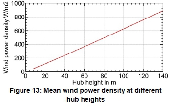
According to this requirement, all months except May and June were in the domain of suitable months for wind farms. This domain could be further extended by taking higher hub heights, as shown in Figure 12. The optimum hub height in Durban is expected to be around 85 m as shown in Figure 13. Therefore, compared to other windy areas, wind power installation in Durban might be more expensive.

 

 

 

 

5. Conclusions

This paper presented the characterisation of wind speed series and power in Durban using Markov chain and Weibull distribution. In developing the Markov model, the measured wind speed series were categorized into sixteen distinct states, and a TPM was formed. This TPM along with its limiting probability vector was used to write a MATLAB code that generates synthetic wind speed series. The median, mean, and standard deviation of the synthetic series are close to those of the measured ones, indicating the accuracy of the model. On the other hand, the shape and scale factors of a Weibull distribution were generated using the measured wind speeds and maximum likelihood estimation method. Comparing the PDFs of the Weibull fit and the Markov model using RMSE methods showed that the latter accurately characterised the wind speed series. Intermediate wind speeds between hours and minutes were also generated using Weibull and Gaussian distributions employing the results of the Markov model. The Markov model can, indeed, generate synthetic wind speeds, which can be used in analysis and simulations of the dynamic behaviour of wind turbines. It can also predict wind speeds for different time horizons. Finally, the analysis of wind power density revealed that large wind turbines having hub heights greater than 85 m could be effective in Durban and its environs. However, compared to windy areas, wind turbines in this area will have high hub heights. In future, larger geographical areas of South Africa, including wider datasets, will be addressed.

 

Acknowledgements

The authors are grateful to the South African Weather Services for providing them with the wind speed data of Durban from 2014 to 2015.

 

References

[1] Asif, M. and Muneer, T. Energy supply, its demand and security issues for developed and emerging economies, Renewable and Sustainable Energy Reviews, 2007, 11: 1388-413, 2007.         [ Links ]

[2] Pimentel, D., Herz, M., Glickstein, M., Zimmerman, M., Allen, R., Becker, K., Evans, J., Hussain, B., Sarsfeld, R., Grosfeld, A. and Seidel, T. Renewable Energy: Current and Potential Issues, BioScience, 2002, 52(12):1111-1120.         [ Links ]

[3] Herberta, G., Iniyan, S., Sreevalsan, E. and Rajapandian, S. A review of wind energy technologies, Renewable and Sustainable Energy Reviews, 2007, 11: 1117-1145.         [ Links ]

[4] Feijóo, A. and Villanueva, D. Assessing wind speed simulation methods, Renewable and Sustainable Energy Reviews, 2016, 56: 473-483.         [ Links ]

[5] Goudarzi, A., Davidson, I. E., Ahmadi, A. and Venayagamoorthy, G. K. Intelligent analysis of wind turbine power curve, in IEEE Symposium on Computational Intelligence Applications in Smart Grid (CIASG) 2014: 1-7.         [ Links ]

[6] Slootweg, J. G. Wind power modelling and impact on power system dynamics, 2003, Ridderkerk, the Netherlands: Delft University of Technology.         [ Links ]

[7] Safari, B. Modeling wind speed and wind power distributions in Rwanda, Renewable and Sustainable Energy Reviews, 2011, 15: 925-935.         [ Links ]

[8] Zárate-Minano, R., Anghel, M. and Milano, F. Continuous wind speed models based on stochastic differential equations, Applied Energy, 2013, 104: 42-49.         [ Links ]

[9] Lei, M., Shiyan, L., Chuanwen, J., Hongling, L. and Yan, Z. A review on the forecasting of wind speed and generated power, Renewable and Sustainable Energy Reviews, 2009, 13 (4): 915920.         [ Links ]

[10] Nfaoui, H. Essiarab, H. and Sayigh, A. A stochastic Markov chain model for simulating wind speed time series at Tangiers, Morocco, Renewable Energy, 2004, 29: 1407-1418.         [ Links ]

[11] Freris, L. Wind energy conversion systems, 1990, Cambridge, UK: Prentice Hall.         [ Links ]

[12] Arslan, T., Bulut, Y. M. and Yavuz, A. A. Comparative study of numerical methods for determining Weibull parameters for wind energy potential, Renewable and Sustainable Energy Reviews, 2014, 40: 820-825.         [ Links ]

[13] Mohammadi, K., Alavi, O., Mostafaeipour, A., Goudarzi, N. and Jalilvand, M. Assessing different parameters estimation methods of Weibull distribution to compute wind power density, Energy Conversion and Management, 2016, 108: 322-335.         [ Links ]

[14] Romero-Ternero, V. Influence of the fitted probability distribution type on the annual mean power generated by wind turbines. A case study at the Canary Islands, Energy Conversion and Management, 2008, 49(8): 2047-2054.         [ Links ]

[15] Carta, J. and Mentado, D. A continuous bivariate model for wind power density and wind turbine energy output estimations, Energy Conversion and Management, 2007, 48(2): 420-432.         [ Links ]

[16] Chang, T. Estimation of wind energy potential using different probability density functions, Applied Energy, 2011, 88(5): 1848-1856.         [ Links ]

[17] Hu, J. and Wang, J. Short-term wind speed prediction using empirical wavelet transform and Gaussian process regression, Energy, 2015, 93: 1456-1466.         [ Links ]

[18] Qin, Z. Li, W. and Xiong, X. Estimating wind speed probability distribution using kernel density method, Electric Power Systems Research, 2011, 81(12): 2139-2146.         [ Links ]

[19] Shokrzadeh, S. Jozani, M. J. and Bibeau, E. Wind turbine power curve modeling using advanced parametric and nonparametric methods, IEEE Transactions on Sustainable Energy, 2014, 5(4): 1262-1269.         [ Links ]

[20] Kazemi, M. and Goudarzi, A. A novel method for estimating wind turbines power output based on least square approximation, International Journal of Engineering and Advanced Technology, 2012, 2(1): 97-101.         [ Links ]

[21] Villanueva, D. and Feijóo, A. A genetic algorithm for the simulation of correlated wind speeds, International Journal of Electrical Power and Energy Systems, 2009, 1(2): 107-112.         [ Links ]

[22] Shamshad, A. Bawadi, M., Hussin, W., Majid, T. and Sanusi, S. First and second order Markov chain models for synthetic generation of wind speed time series, Energy, 2005, 30: 693-708.         [ Links ]

[23] Kantza, H., Holsteina, D., Ragwitzb, M. and Vitanov, N. K. Markov chain model for turbulent wind speed data, Physica A, 2004, 342: 315-321.         [ Links ]

[24] Ettoumi, F. Y., Sauvageot, H. and Adane, A. Statistical bivariate modeling of wind using first-order Markov chain and Weibull distribution, Renewable Energy, 2003, 28: 1787-1802.         [ Links ]

[25] D'Amico, G., Petroni, F. and Prattico, F. First and second order semi-Markov chains for wind speed modeling, Physica A, 2012, 392: 1194-1201.         [ Links ]

[26] Otto, A. Wind Atlas For South Africa, June 2004, SANEDI.         [ Links ]

[27] Herbst, L. and Lalk, J. A case study of climate variability effects on wind resources in South Africa, Journal of Energy in Southern Africa, August 2014, 2-10.         [ Links ]

[28] Mosetlhe, T. C., Yusuff, A. A., Hamam, Y. and Jimoh, A. A. Estimation of wind speed statistical distribution at Vredendal, South Africa, International Journal of Power and Energy Systems, 2016, DOI: 10.2316/P.2016.839-017.         [ Links ]

[29] Heier, S. Grid integration of wind energy conversion systems, 2005, Chichester: John Wiley & Sons.         [ Links ]

[30] Meyn, S. and Tweedie, R. Markov chains and stochastic stability, 2005: Springer-Verlag.         [ Links ]

[31] Hocaoglu, F. O., Gerek, O. N. and Kurban, M. The Effect of Markov Chain State Size for Synthetic Wind Speed Generation, in Proceedings of the 10th International Conference on Probabilistic Methods Applied to Power Systems, 2008. PMAPS '08.         [ Links ]

[32] Scott, M. Characterizations of strong ergodicity for continuous time Markov chains, 1979, PhD thesis: Iowa State University Ames.         [ Links ]

[33] Aksoy, H., Toprak, Z. F., Aytek, A. and Unal, N. E. Stochastic generation ofhourly mean wind speed data, Renewable Energy, 2004, 29: 2111-2131.         [ Links ]

[34] Agustín, E.-S. C. Estimation of Extreme Wind Speeds by Using Mixed Distributions, Ingeniería, Investigación y Tecnología, 2013, 14(2): 153-162.         [ Links ]

[35] Datta, R. and Ranganathan, V. T. A method of tracking the peak power points for a variable speed wind energy conversion system, IEEE Transaction on Energy Conversion, 2003, 18(1): 163-168.         [ Links ]

[36] Ramachandra, T., Subramanian, D. and Joshi, N. Wind energy potential assessment in Uttarannada district of Karnataka, India, Renewable Energy, 1997, 10(4): 585-611.         [ Links ]

[37] Bhaskar, B. Energy Security and Economic Development in India: a holistic approach, The Energy and Resources Institute (TERI), 2013.         [ Links ]

 

 

* Corresponding author: Tel: +27 31 260 2725; Email: 214584668@stu.ukzn.ac.za or ayelenigussie@yahoo.com