ARTICLES

 

Power calculation accuracy as a function of wind data resolution

 

 

Martinus Gerhardus de Klerk^*; Willem Christiaan Venter

Department of Electrical, Electronic and Computer Engineering, North-West University, Private Bag X6001, Potchefstroom, 2520

 

 

---

ABSTRACT

Wind power calculations are usually based on average wind data taken over one-hour intervals. The effect of the wind data resolution on the statistical techniques used to calculate the probable power output (PPO) is commonly overlooked. This effect is analysed in this paper by iteratively calculating and comparing the PPO of a wind turbine using data, averaged over different periods, obtained from Wind Association of South Africa. The power is calculated using both Weibull representation and direct polynomial substitution techniques in order to compare and verify the results. The results indicate a fairly linear relationship between the resolution used and the PPO error incurred. These results raise an interest to examine the effects of a fine resolution on the data in terms of data dependence, which may violate the criteria for the majority of statistical tests and procedures.

Keywords: data resolution analysis, wind power, Weibull

---

 

 

1. Introduction

An ever-increasing demand for energy exists today, especially utilising clean renewable energy sources. Although such sources are available, an accurate analysis of their feasibility is required before deciding to harness these sources at specific locations. The focus of this article pertains to wind energy as a renewable energy source. When considering a location for harnessing of wind energy, the PPO of a wind turbine subjected to the wind present at that location must be determined from historical wind data recorded there. It is commonly assumed that wind data with an hourly resolution will be adequate for these calculations, without giving further attention to the compounding effect that the data resolution has on additional calculations. This article presents an investigation into the power calculation's accuracy based on the wind data resolution. The investigation entails the PPO calculation for a given site and wind turbine for various resolutions of the data. The results are then analysed to determine the impact of the wind data resolution on the results.

Wind data generally provides the speed and direction in which the wind is blowing for a given period of time. Wind data is influenced by the geographical environment, be it natural or man-made, as well as the height at which it is measured. The variable nature of wind tends to makes it a cumbersome resource to measure, represent and analyse. Wind data sets analysis for various locations and heights in this investigation were used in order to perform an unbiased analysis of the data resolution's effect. The wind data sets used were obtained from the Wind Association of South Africa (WASA), an initiative between the South-African government and the Department of Energy. The Association is financially supported by the Royal Danish Embassy as well as the United Nations Development Program - Global environment facility (UNDP-GEF) through the South African Wind Energy Program (Wind Atlas for South Africa, 2014). The WASA project gathers data from 10 sites around South Africa, situated on both the coast and inland, as listed in Table 1.

 

 

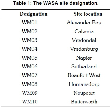
Each site records wind speed data at heights of 10m, 20m, 40m, 60m and 62m by saving the average for each 10-minute interval in comma-separated value (.csv) files.

In this raw form, the wind speed data is merely an estimator of what the average wind speed was during the measuring period. This in itself is not enough to quantise the availability of wind, which is further complicated by the variable nature thereof. In order to overcome this quantising problem, statistical techniques can be employed for data distribution, and in doing so, make the data more intelligible and easier to work with. One of the simplest ways to obtain a meaningful representation of the data is by means of a histogram. When drawing a histogram of the wind speed data, using an adequate bin width Ax one is left with a distribution showing how many observations fall within each bin, essentially providing an estimation of the probability distribution of the data as shown in Figure 1. An adequate bin width is dependent on the number of bins k required to represent the distribution of the data. This is usually determined by experimentation, but Sturges' formula (Lane & University 2006) can also be employed according to Equation 1.

 

 

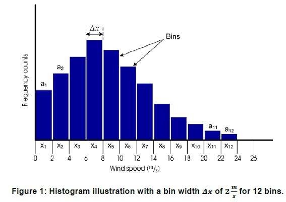
where n is the number of observations. This will provide a reference value, but may need some adjusting since Sturges' formula assumes an approximately normal distribution (Vose Software 2007).

When employing Sturges' rule on the wind data from the test site WM01 in Alexander Bay for a month with 31 days, it amounts to an n = (6 X 24 X 31) = 4464, based upon a wind data intervals of 10 minutes, suggesting to use k = 13.1241 ≈ 14 bins for the histogram as illustrated in Figure 2. This implies that the wind data is grouped in 14 bins, ranging from to a value encapsulating the maximum wind speed found in the wind data set, in this case 0 to 28 with wind speeds grouped in bins.

 

 

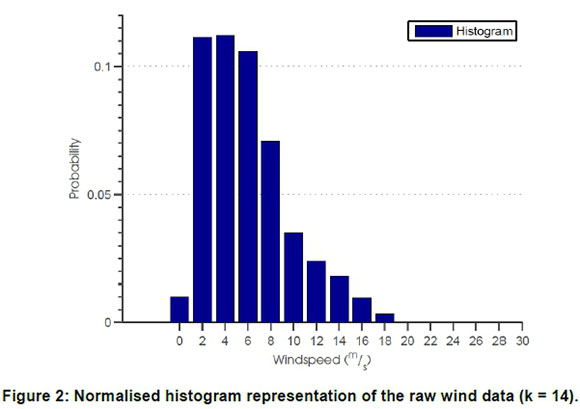
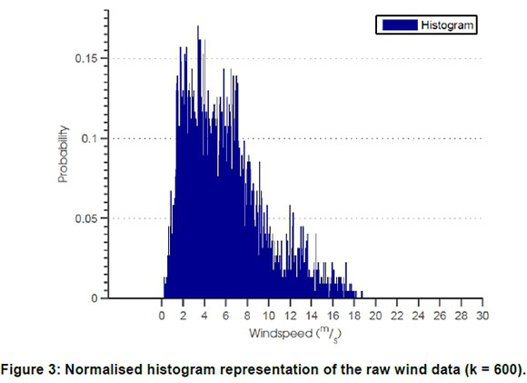
Figure 3 illustrates a histogram of the same data with k = 600.

 

 

The wind data from test site WM01 can also be approximated by means of the Weibull probability density function (PDF). The Weibull distribution, generated by the Weibull PDF, performs a task similar to a histogram, but surpasses it by smoothing the data and allowing the data to be easily represented by means of a simple equation. The Weibull distribution is particularly well suited to failure rates (Hayter, 2012) as well as to provide a close approximation to the probability laws of many natural phenomena (Lun & Lam, 2000).

The Weibull distribution provides a statistical distribution depicting the probability of encountering each possible outcome of a random experiment, in this case the probability of encountering a certain wind speed based on long-term meteorological data. The Weibull PDF does not provide only the average wind speed, but also the probability of encountering each wind speed. This wind speed probability will later be used to determine the probable power output of wind turbines. The Weibull PDF is expressed as in Equation 2.

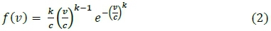
where k is a dimensionless shape parameter and c the scale parameter with the same unit as the wind speed v (Lun & Lam 2000). Once the Weibull curve has been generated for a given data set, it will provide a mathematical representation of the data distribution, hence speeding up calculations and freeing up memory by representing the actual data set, no matter how large it was initially. Histograms are generally graphed using bars to represent each bin, but in Figure 4 the values have been graphed using a normal line plot in order to compare it with the Weibull distribution of the wind data. It is clear from Figure 4 that the Weibull probability function provides a good representation of the raw wind data (Carrillo et al. 2014).

The Weibull PDF will be used to represent the wind speed probability when performing PPO calculations. The accuracy of a Weibull distribution depends on the parameters used in the Weibull PDF. There are various methods that can be used to determine the values of the shape and scale parameters, each with their respective pros and cons (Al-Fawzan, 2000).

The maximum likelihood estimation (MLE) method is commonly used in literature to determine the shape and scale parameters for the Weibull function and consists of two equations.

The shape parameter k of the wind data can be calculated by iteratively implementing Equation 3 (Seguro & Lambert, 2000):

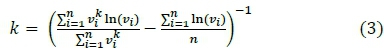
with an initial estimate of k = 2. Each wind speed v from the data set with n observations is indexed by i. A shape parameter of k = 2 is used as an initial guess since it represents a special case of the Weibull distribution, namely the Rayleigh distribution, which provides a fairly typical curve for many locations (Burton et al. 2011). It is important to note that this method only functions with non-zero data values. Since the aim is to model the available wind speeds, the zero values were omitted for these tests.

Subsequently the scale parameter c can be calculated by Equation 4.

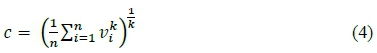
The MLE method is asymptotically consistent, implying that the parameter estimates converges to the right values as the sample size increases. The method may, however, not be very accurate with small sample sizes (Hatahet, 2006). As a rule of thumb, a small sample size is defined as less than 30 observations per parameter (University of California Regents, 2003).

The MLE is a fairly computational intensive task, especially as the size of the data sets increases. Alternative methods for parameter estimation were also considered. LabVIEW provides an alternative method to estimate the shape and scale parameters of the Weibull curve representing the wind data called a curve fit method (CFM). This alternative method requires a histogram to be created with adequate bin width as described in section 3.1. Afterwards the histogram's data is supplied to the nonlinear curve fit virtual instrument (VI) along with common shape and scale parameter values, in this case a value of 2 for both parameters. The non-linear curve fit VI uses the Levenberg-Marquardt algorithm to determine the set of Weibull PDF parameters that provide the best fit for the set of input data points (National Instruments 2008).

The parameter estimation time becomes quite lengthy due to the magnitude of the data sets used in the analysis. The average number of data entries used for these calculations, based on a resolution of λ = 1 = 10 rain adds up to 4 464 data entries for a 31 day month, averaging 52 560 data entries per year, per site.

Substantially fewer data entries are left that need to be analysed when representing the data set in the form of a histogram. This allows the CFM to estimate the Weibull curve's parameters faster than the MLE when supplied with large data sets with only a slight compromise in accuracy due to the smoothing characteristics of the Weibull curve used to approximate the data's histogram. The computational times for the MLE and CFM are compared in Table 2, based on a case study using the data from WASA's WM01 site based in Alexander Bay. The CFM produced the parameters much faster than the MLE method - in this case approximately 280 times faster.

 

 

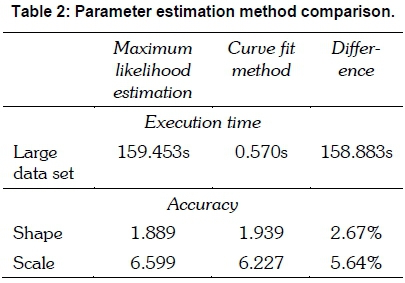
The MLE method is considered to be the more accurate method to determine the parameters of the Weibull distribution. The parameters of the CFM in this analysis, however, differ at most by 5.64% from the parameters of the MLE method. Taking the execution speed into account, it was decided to use the CFM to calculate the parameters of the Weibull distribution in this investigation.

With the wind speed data represented in an intelligible manner, the focus can shift to the harnessing of the wind. Wind turbines are devices that convert the kinetic energy of the wind into mechanical energy, which in turns generate electricity with the help of an electric generator. The power created by the electric generator is dependent on the wind speed as well as the wind turbine's technical specifications.

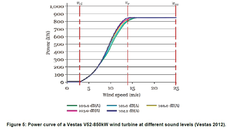
The power curve of a wind turbine displays the power output of the specific turbine configuration for each corresponding wind speed. A wind turbine has four phases of power generation as indicated on the power curve of the Vestas V52-850kW turbine in Figure 5.

• 0 → v_ci no generation;

• v_ci→ v_rmaximum rotor efficiency;

• v_r→ v_conominal power generation with reduced rotor efficiency;

• v_co→ ∞ no generation.

The cut-in speed of the turbine, v_ci, is the minimum speed at which the turbine will start generating power. The range between the cut-in speed and the rated wind speed v_ris generally proportionate to the cube of the wind speed (v³). The optimal power producing operational phase of the wind turbine is in the range between the rated wind speed v_rand the cut-out speed v_cowhere the wind turbine will produce its rated power output. It is important to note that when the wind speed is greater than the cut-out speed the turbine ceases to produce power as a safety precaution in order to prevent over-powering of the infrastructure.

An accurate mathematical representation of the turbine's power curve can be obtained by fitting a polynomial curve to the manufacturer's power curve. The MATLAB simulations and polynomial fitting in Microsoft Excel showed that a sixth-order polynomial, as shown in Figure 6, provides the best approximation of the manufacturer's power curve as illustrated in Figure 5.

 

 

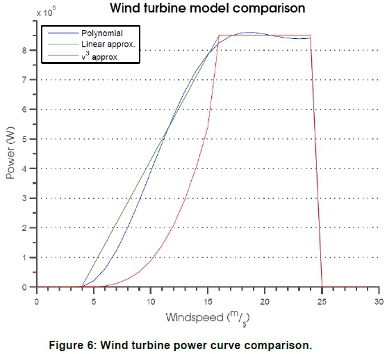
The equation of a sixth-order polynomial is given by Equation 5.

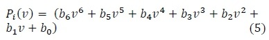
where b_tε R for any i ε Z⁺.

The calculated Weibull distribution of the wind speeds can be applied to determine the PPO of wind turbines. This can be approached by calculating the theoretical amount of power available in the wind and then how much of that power can be extracted by a wind turbine based on its dimensions.

The theoretical power P available in the wind can be expressed as in Equation 6 (Ramírez & Carta, 2005).

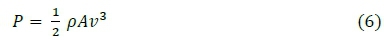
where p is the density of air that flows perpendicular to an area A (m²) with a velocity

It is important to note that the density of air varies with altitude and temperature. When using Equation 6 to calculate the theoretical power available in the wind, the Lanchester-Betz limit has to be taken into account. The Lanchester-Betz limit states that the maximum power that can be extracted from the wind is 59.3% of the power available in the wind under ideal conditions (Cuerva & Sanz-Andrés, 2005).

It is, however, possible to calculate the probable power output P_prob, (v) of a wind turbine without calculating the Lanchester-Betz limit because the wind turbine's power curve relates wind speed to power output and can be calculated in one of two ways. The first method, known as the polynomial substitution, is computationally intensive. Each wind speed data entry is supplied to the wind turbine power curve polynomial and the final result is averaged as in Equation 7.

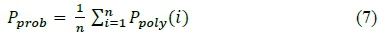
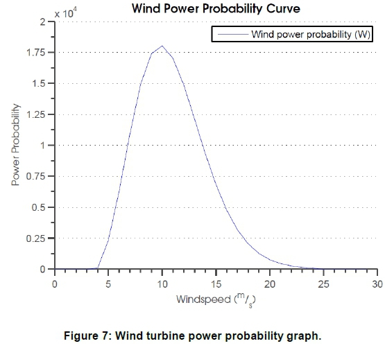
where n is the number of entries in the wind speed data set and P_poly (i) is the turbine power curve polynomial, in this case given by Equation 9, which is addressed later. An alternative method is to make use of the Weibull PDF, which provides the probability of each wind speed being present as shown in Figure 4, while the power curve indicates the power that will be available at each wind speed shown in Figure 6. These two graphs can be multiplied to obtain a wind turbine power probability graph (Bradbury, 2008), as illustrated in Figure 7.

 

 

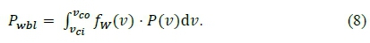
Thus, following the calculation of the Weibull curves f_w (v) and the turbine power curve P(v), the probable power output can be calculated in terms of Equation 8.

The polynomial substitution provides a more accurate depiction of the average PPO since raw data was used and not smoothed data as with the Weibull curve and its associated parameter estimation techniques. The latter method is advantageous because of its processing speed. Once the Weibull curves were generated, the wind turbine's parameters can be changed and the probable power output can be calculated almost instantaneously by implementing Equation 8, while Equation 7 would require re-evaluation of the power polynomial for every single data entry.

 

2. Methodology for analysing the wind data resolution

The effect of the wind data's resolution thereon can be determined with an established methodology for the calculation of the PPO of a wind turbine. The wind data resolution is a measure of the observation frequency at which the data is logged. It is widely accepted that a data resolution of one- hour intervals provides satisfactory accuracy when working with wind data (Protogeropoulos, 1992). The goal of the analysis in this investigation is to determine the effect of the wind data resolution on the accuracy of subsequent power calculations.

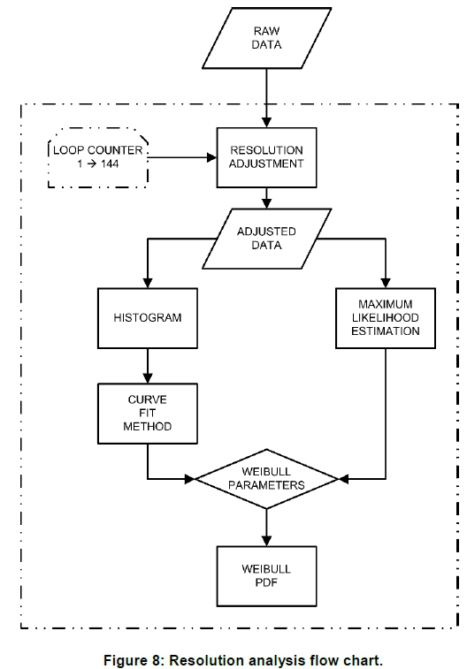
The effect of the resolution on the power calculations can be determined by keeping all variables constant, with an exception of the wind data's resolution. This process flow is shown in Figure 8, where LabVIEW was used to calculate the Weibull parameters of the wind data for each resolution interval. The Weibull parameters for each resolution interval were calculated using both the MLE and the CFM techniques to verify the results.

 

 

In the next step, the PPO of the wind turbine was calculated using the sixth-order polynomial turbine power curve. The Weibull parameters of the input data in this step, calculated as described in the previous paragraph were used. A baseline value for the PPO was calculated by substituting each wind speed data value into the sixth-order power curve polynomial in Equation 9, for the Vestas V52-850 kW wind turbine (Vestas, 2012) and averaging all these values as given by Equation 7.

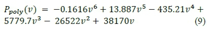
The constant values of the polynomial in Equation 9 were calculated by fitting a sixth-order polynomial through the manufacturer's power curve. The polynomial provides a good representation of the transient phase and most of the rated phase of the wind turbine's power curve, but it is important to enforce the cut-in and cut-out velocities of the turbine explicitly in the models (Weibull PDF and polynomial substitution).

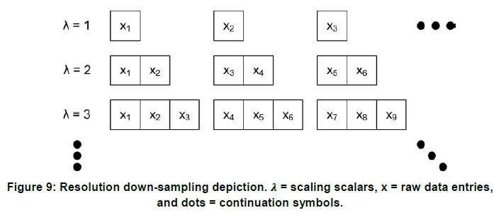
The raw wind data set consists of data entries representing the average wind speed over 10-mi-nute intervals, i.e., λ = 1, where λ is a scalar value ranging from 1 - 144 and where 1 represents the 10-minute intervals and 144 represents a period of 24 hours. A new resolution data set was created by down-sampling and averaging data entries from the raw data set. This is graphically depicted in Figure 9, where x_tdenotes the raw data entries where i = {1,2,3,...}.

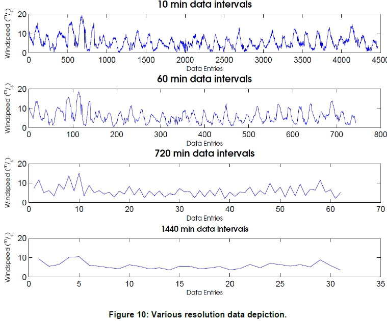
The effect of this down sampling process is shown in Figure 10 where the raw data resolution of λ = 1 is shown alongside λ = 6 (hourly), λ = 72 (every 12 hours), and λ= 144 (daily) intervals.

 

3. Results

The analysis of the power calculation accuracy as a function of the wind data resolution is split into different sections. Each section investigates the impact of a different part of the process followed. To start with, it is important that the impact of the resolution and data representation techniques on the power calculations must be kept in mind. As λ increases, the number of available data entries decreases by the same factor. This reduces the MLE iterations, which is not advantageous since the MLE algorithm becomes less accurate as a result thereof. This is also true about the reduced observations available for the histogram in the CFM, which ultimately results in less accurate representation of the raw data set. The CFM, however, is less dependent on the number of observations in the histogram since it is only reliant on the envelope of the histogram.

As already discussed, the Weibull distribution is the preferred method of representation for the wind data. The Weibull distribution is also used for the PPO calculation because of its simplicity. Both the MLE and the CFM techniques can be used to calculate the shape and scale parameters of the Weibull distribution. It can be shown that the shape and scale parameters calculated with both the MLE and CFM techniques correlate fairly well with each other as shown in Table 3. Data used in this case study was with a resolution of λ = 1 ≈ 10 minutes from site WM-01 (Alexander Bay) at a height of 62 m.

From Table 3 it can be seen that both parameter estimation techniques produce fairly similar results for the shape and scale parameters of the Weibull distribution when applied to the same data. The maximum difference between the MLE and CFM parameters was found in July with a value of 9.718%.

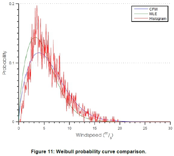
In the next step Weibull curves were generated using the shape and scale parameters of both the MLE and CFM techniques as previously discussed. Comparing these Weibull curves with the histogram of the raw data used in the calculations, it became apparent that these Weibull curves were a good representation of the raw data as illustrated in Figure 11.

 

 

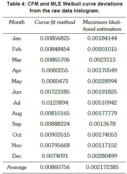
The average differences between the raw data's normalised histogram and the Weibull curves are listed in Table 4. It was decided to use Weibull curves based on MLE calculations in the rest of the investigation because of the simplicity of Table 4.

 

 

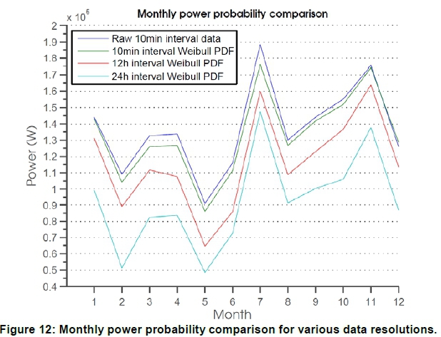
The next parameter, the effect of the wind data resolution on the PPO calculations, was investigated. The PPO was calculated using Weibull curves and the turbine power curve as expressed in Equation 8. A Weibull distribution created from aforementioned MLE parameters was used. It was found that there was a clear difference between the mean power output in each month depending on the resolution of the wind data used. An almost linear shift between the PPOs calculated using wind data with different resolutions can be seen in Figure 12. The coarser the wind data resolution, the lower the PPO observed across all months. The PPO difference is not the exact same amount for each month, but indicates a fairly linear shift relative to the resolution used.

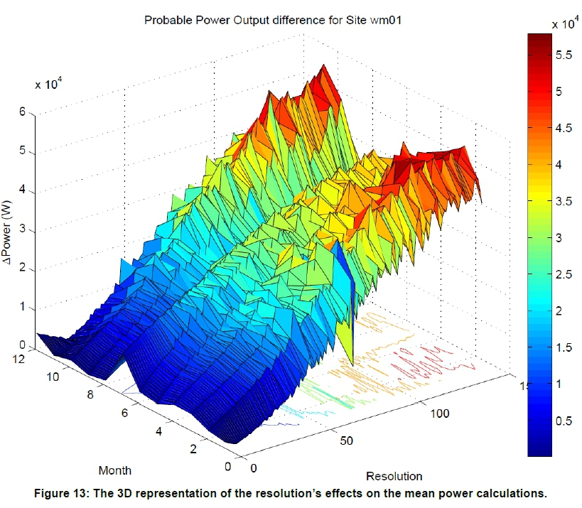
The extent of the resolution's effect on the PPO calculated as mentioned above was determined by a contrast to another PPO calculation. The most accurate, but time-consuming, PPO calculation (P_poly) was done by direct substitution of the raw data into Equation 9. The PPO difference P_diffbetween the two approaches were calculated by Equation 10.

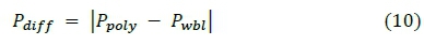
where P_wbl is the aforementioned Weibull PPO.

This difference can be seen in Figure 13 for each month as a function of the resolution used. The finer the resolution used for the calculations, the smaller the PPO difference observed.

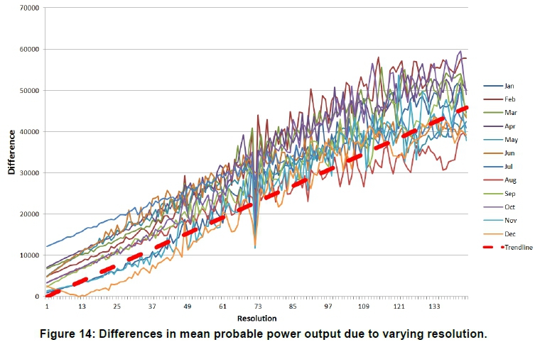
An anomaly was observed at certain resolutions during the resolution analysis and can be seen in Figure 14 where, at a resolution of λ = 72, there is a prominent drop in the observed PPO differences across all months. A smaller anomaly was observed at = 48 , which was only when an increase in the PPO differences was recorded.

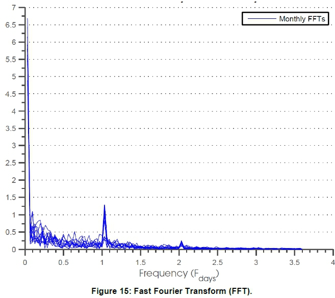
Similar results were also obtained using a different data set. Seasonality in the wind data was to be expected, but after calculating the Fast Fourier Transform (FFT) of the raw data for various months, a notable discovery was made. The FFT of the various months are overlaid in Figure 15 to highlight any similarities between the different months. It is clear from Figure 15 that harmonics were present in the data. The peak located at a frequency of one day was expected, but there seems to be a prominent harmonic at a frequency of two - i.e. every 12 hours (λ = 72). This correlated with the abnormality found in Figure 14. Following this trend, another peak as expected at a frequency of three, i.e., every eight hours correlating with the abnormality at λ = 48, but was associated with too much noise on the graph to make a definitive inference.

As previously stated, the mean monthly power difference for the various resolutions are illustrated in Figure 14.

 

4. Conclusions

The investigation in this article leads to the conclusion that wind data resolution has a prominent effect on the PPO calculation of a wind turbine: the coarser the wind data used, the larger the error in the PPO calculation. The assumption that wind data of an hourly resolution could be used for calculations must, therefore, always be done in consideration to this error. The hourly averaged wind data's PPO results differed by approximately 2.51% from the results obtained by the polynomial substitution. From the results obtained during this investigation, the following hypothesis was drawn: The error in the power output calculation of a wind turbine generator is linearly related to the resolution of the wind data used for the calculation.

It was clear that the resolution of the wind speed data had a substantial effect on the accuracy of all relevant power probability calculations. Further investigation can be done into what effect a fine resolution has on the data in terms of data dependence, which may violate the criteria for the majority of statistical tests and procedures (Ramirez & Carta, 2005). The nature of the aforementioned anomaly also warrants further investigation. Furthermore, it might be beneficial to investigate the effect of turbulence intensity on power calculations.

 

Acknowledgements

The authors thank the Wind Atlas for South Africa for providing the data, as well as the Department of Science and Technology for subsidising the project.

 

References

Al-Fawzan, M.A. 2000. Methods for estimating the parameters of the Weibull distribution. King Ab- dulaziz City for Science and Technology, Saudi Arabia.         [ Links ]

Bradbury, L. 2008 Wind-power program. Available at: http://www.wind-power-program.com/mean_power_calculation.htm.         [ Links ]

Burton, T., Jenkins, N., Sharpe, D. and Bossanyi, E. 2011. Wind energy handbook (2nd ed). Wiley.         [ Links ]

Carrillo, C., Cidras, J., Diaz-Dorado, E. and Obando-Montano, A.F. 2014. An approach to determine the Weibull parameters for wind energy analysis: The case of Galicia (Spain). Energies 7(4): 2676-2700.         [ Links ]

Cuerva, A. and Sanz-Andrés, A. 2005. The extended Betz-Lanchester limit. Renewable Energy 30(5): 783-794. Available at: http://linkinghub.elsevier.com/retrieve/pii/S0960148104002885 [Accessed April 28, 2012].         [ Links ]

Hatahet, Z. 2006. Wind data analyzer, Internship Report at Hochscule Wismar, Germany, Toronto, Canada.         [ Links ]

Hayter, A. 2012. Probability and statistics for engineers and scientists (4th ed). Boston, MA: Brooks / Cole.         [ Links ]

Lane, D.M. and University, R., 2006. Online statistics education: An interactive multimedia course of study. Available at: http://onlinestatbook.com/2/graphing_distributions/histograms.html.         [ Links ]

Lun, I.Y. and Lam, J.C. 2000. A study of Weibull parameters using long-term wind observations. Renewable Energy 20(2): 145-153. Available at: http://linkinghub.elsevier.com/retrieve/pii/S0960148199001032.         [ Links ]

National Instruments, 2008. National instruments. Available at: http://www.ni.com/white-paper/6954/en/.         [ Links ]

Protogeropoulos, C.I. 1992. Autonomous wind / solar power systems with battery storage. University of Wales College, Cardiff, Wales.         [ Links ]

Ramírez, P. and Carta, J.A. 2005 Influence of the data sampling interval in the estimation of the parameters of the Weibull wind speed probability density distribution: A case study. Energy Conversion and Management 46(15-16): 2419-2438. Available at: http://linkinghub.elsevier.com/retrieve/pii/S0196890404003036 [Accessed March 22, 2012].         [ Links ]

Seguro, J.V. and Lambert, T.W. 2000 Modern estimation of the parameters of the Weibull wind speed distribution for wind energy analysis. Journal of Wind Engineering and Industrial Aerodynamics 85(1), 75-84. Available at: http://linkinghub.elsevier.com/retrieve/pii/S0167610599001221.         [ Links ]

University of California Regents, 2003. Maximum likelihood procedures. Available at: http://elsa.berkeley.edu/sst/max.like.html.         [ Links ]

Vestas, 2012. Vestas V52., p.6. Available at: http://pdf.directindustry.com/pdf/vestas/v52-850-kw-brochure/20680-53603-_3.html.         [ Links ]

Vose software, 2007. Vose software - Risk software specialists. Available at: http://www.vosesoftware.com.         [ Links ]

South African National Energy Development Institute, 2014. Wind Atlas for South Africa. Department of Energy of South Africa, 2014. Available at: http://www.wasaproject.info/about_wind_energy.html [Accessed January 1, 2016].         [ Links ]

 

 

* Corresponding author: Tel: +27 79 523 6579 Email: gdknwu@gmail.com; 20555466@nwu.ac.za)