ARTICLES

 

Quantifying South Africa's sulphur dioxide emission efficiency in coal-powered electricity generation by fitting the three-parameter log-logistic distribution

 

 

Maseapei Elizabeth Girmay^*; Delson Chikobvu

Department of Mathematical Statistics and Actuarial Science, University of the Free State, PO Box 339, Bloemfontein 9300, South Africa

 

 

---

ABSTRACT

This paper fits the three-parameter log-logistic (3LL) distribution to sulphur dioxide (SO2) monthly emissions in kilograms per gigawatt hour (kg/GWh) and in milligrams per cubic nano metre (mg/Nm³), at 13 of Eskom's coal fired power-generating stations in South Africa. The aim is to quantify and describe the emission of sulphur dioxide at these stations using a statistical distribution, and to also estimate the probabilities of extreme emissions and exceedances (emissions above a certain threshold). Using the 3LL distribution is proposed as such a distribution. The log-logistic distribution is a special form of a Burr-type distribution. Various goodness-of-fit measures, including the Kolmogorov Smirnov, the Anderson Darling and some graphical tests, are employed to test if the 3LL distribution is a good fit to the data. The maximum likelihood method is used to estimate the parameters. The distribution fit is important as it then becomes possible to quantify and manage the SO₂ emissions effectively. The 3LL distribution, which is compared with three other distributions, gave the best overall fit to most of the power stations.
Highlights
• Quantification of SO₂ emissions in terms of a statistical distribution
• Calculating the probability of SO2 emissions exceeding certain specified limits
• Ranking power stations in terms of SO2 emissions efficiency

Keywords: emission, Eskom, log logistic distribution, goodness of fit, sulphur dioxide, Burr-type distribution

---

 

 

1. Introduction

Eskom is South Africa's electricity public utility, established in 1923 as the Electricity Supply Commission by the government of South Africa. It is the largest producer of electricity in Africa, and among the top seven utilities in the world in terms of generation capacity and among the top nine in terms of sales. Eskom generates approximately 95% of electricity used in South Africa. About 95% of its generating capacity comes from coal. Ash emissions from Eskom's coal-fired power stations have been reduced by more than 90% since the early 1980s due to the installation of efficient pollution abatement technology and the decommissioning of older plants (Eskom Emission Monitoring, 2012). At present, Eskom has 13 coal-fired generating stations giving various emissions, including sulphur dioxide (SO₂). Medupi and Kusile are two new stations and are not included in the analysis.

Coal-fired power stations release harmful chemicals (stack emissions) into the atmosphere, causing environmental problems. Sulphur dioxide, for example, is a precursor to acid deposition (including acid rain) and secondary particulate matter formation, and is also toxic. Eskom must comply with legally prescribed limits on a number of emissions to avoid heavy penalties. Exceeding the emission limits may result in the forced shutdown of generating units. Emission levels must therefore be monitored and alarmed continuously. A stack test is a procedure for sampling a gas stream from a single sampling location at a facility, unit, or pollution control equipment. Each of Eskom's stations could be a unit, and there could also be more than one unit at a station. The stack is used to determine a pollutant emission rate, concentration, or parameter while the facility, unit, or pollution control equipment is operating at conditions that result in the measurement of the highest emission or parameter values (prior to any control device) or at other operating conditions approved by the regulatory authority. Stack emission control programmes are effective only if emissions are controlled at the source, which requires a highly accurate monitoring schedule. Stack emissions are measured for various reasons, including to determine if emission permits requirements are met or exceeded, for emissions permit renewal, or for process control purposes. Reporting on environmental performance has several benefits, including providing management with information to help exploit the cost savings that good environmental performance usually brings; it also gives Eskom the chance to set out what they believe is significant in their environmental performance. Companies that measure (to quantify), manage and communicate their environmental performance are inherently well placed. They understand how to improve their processes, reduce their costs, comply with regulatory requirements and stakeholder expectations, and take advantage of new technologies on the market. This paper describes SO2 emissions at 13 Eskom coal-fired power stations measured by fitting a three-parameter log-logistic (3LL) distribution. The maximum likelihood method is used to estimate the parameters. The 3LL is compared with three other distributions, namely the normal, log-normal and three-parameter Weibull. A literature review follows in Section 2; methodology is outlined in Section 3; the data and results are given in Section 4 and conclusions in Section 5.

 

2. Literature review

Little if any modelling of pollutant emissions in South Africa is done. Geogopolous et al. (1982) stated that the answer to the question of which distribution best fits the air quality/emissions data was shown to depend in general on the pollutant, the time period of interest, the averaging time of the data, the location and other factors. Generally there is no priori reason to choose one particular distribution over the other (Seinfeld et al., 1998). Yi Zhang et al. (1994) investigated the statistical distribution of on-road carbon monoxide and hydrocarbon emissions from various locations in the United States, and found that the emissions are statistically gamma-distributed. Rumburg et al. (2001) investigated the statistical distribution of particulate matter in Spokane, Washington and concluded that the distribution was best fitted by a three-parameter lognormal distribution and a generalised extreme value distribution. Hadley et al. (2003) investigated the distribution of annual mean daily SO2 in the United Kingdom and found the log-normal distribution to be a better fit for the data than the normal. One of the most important papers on modelling greenhouse gas emissions is that of Smith (1989), where he applies the extreme value theory to the study of hourly readings of ozone in Houston, Texas, since excessive levels of ozone are taken to indicate high air pollution. Smith concluded that the exponential distribution gave a poor fit in the upper tail whereas the generalised Pareto distribution seemed adequate.

The method of estimation of parameters for the chosen statistical distribution is also important when emission data is available. Ashkar et al. (2003) compared the maximum likelihood (ML) and the generalised probability weighted moments (GPWM) in estimating the parameters of a log-logistic, and found that the ML outperformed the GPWM method over all parameter space and sample sizes. Ashkar et al. (2006) compared the method of generalised moments, ML, the methods of the GPWM and the method of log moments for the estimation of the parameters and quantiles in the two-parameter log-logistic. Their simulation results showed that the GM method outperformed the other competitive methods in the two-parameter log-logistic case when the moment orders are appropriately chosen. Abbas et al. (2015) proposed the Bayesian method using the metropolis algorithm within the Gibbs sampling under the reference prior to estimate the parameters of the log-logistic. Singh et al. (1993) developed a new competitive method of estimating parameters of the log-logistic based on the principle of maximum entropy (POME) using the Monte Carlo simulated data, and compared it to the methods of moments (MOM), ML, and the probability weighted moments (PWM). They concluded that POME yielded the least parameter bias for all sample sizes. Other parameter estimation problems for the log-logistic distribution are addressed by, among others, Kantam and Srinivasa (2002), Balakrishnan et al. (1987), and Tiku and Suresh (1992). The log-logistic distribution is a special type of a Burr-type XII distribution. Burr (1942) introduced twelve different forms of cumulative distribution functions for modelling data, of which Burr-type X and Burr-type XII received the maximum attention. There is also a thorough analysis of Burr-type XII distribution in Rodriguez (1977), and see also Wingo (1993). Burr-type distributions are very flexible and can be adapted to fit many situations. In this paper the three-parameter log-logistic distribution from the Burr-type XII family is used. The normal is one of the most commonly used distributions where there is a large data set. Log-normal is one of the distributions commonly mentioned in the literature on emissions; the variance of the log-normal increases with the mean. The three-parameter Weibull distribution is also one of the commonly used reported distributions, and it is also heavy-tailed.

 

3. Research methodology

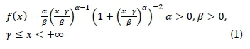
This section describes the statistical distribution used to describe the SO2 emissions data and the method of estimating the parameters. The log-logistic distribution is a continuous probability distribution for a non-negative random variable. It is the probability distribution of a random variable whose logarithm has a logistic distribution. It is generated by a transformation of logistic variable, just like the log-normal distribution is obtained from the normal distribution. It is similar in shape to the log-normal distribution but has heavier tails. The log-logistic distribution is a special case of the Burr-type XII distribution (Burr, 1942) and also a special case of the Kappa distribution (Mielke & Johnson, 1973). The Burr distribution is very relevant in the study of atmospheric emissions, it is more flexible and has heavier tails and is then able to model extreme emissions. Its cumulative distribution function can be written in closed form, unlike that of the log-normal. The 3LL distribution has a probability density function given as in Equation 1.

and a cumulative distribution given by Equation 2:

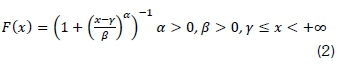
where β > 0is a scale parameter, a > 0is a shape parameter and γ ε R is a location parameter. The distribution is unimodal when the shape parameter a > 1 and its dispersion decreases as the shape parameter a increases.

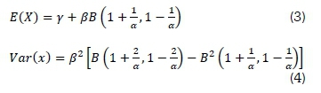
The mean and variance of the 3LL distribution are given by Equations 3 and 4 respectively:

3.1 Parameter estimation

The parameters are estimated using the ML method. The ML is asymptotically normal, has the smallest asymptotic variance, and is asymptotically efficient and optimal. With the ML approach, the distributions of the estimators become more and more concentrated near the true value of the parameter being estimated as the sample size (n) increases.

Maximum likelihood method: The probability density function of the 3LL distribution is given in Equation (1) above, with the log likelihood given in Equation 5:

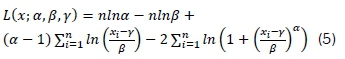
where η is the sample size. Taking the partial derivatives of each parameter gives Equations 6-8:

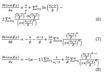
The maximum likelihood estimates â, and are obtained by setting each of the above equations to zero and solving them simultaneously. Optimisation computer algorithms such as the Newton-Raphson, Nelder-Mead, and simulated annealing are often used to arrive at the estimates. The normal, log-normal and three-parameter Weibull distribution parameters are estimated in a similar way.

3.2. Goodness of fit tests

The Anderson-Darling, Chi Squared, and Kolmogo-rov-Smirnov tests are used to test if the 3LL is a good distribution to fit the data. The probability density function (PDF) plots, cumulative distribution function (CDF) plots, together with the probability-probability (P-P) and quantile-quantile (Q-Q) plots are also used as tests.

The Kolmogorov-Smirnov test is a nonparamet-ric test for the equality of continuous, one-dimensional probability or statistical distributions that can be used to compare a sample of observations with a reference probability distribution or to compare two samples. It tries to determine if two data sets differ significantly, and has the advantage of making no assumption about the statistical distribution of data. It quantifies a distance between the empirical distribution function of the sample and the theoretical cumulative distribution function, or between the empirical distribution functions of two samples. The test statistic of the Kolmogorov Smirnov is given by Equation 9:

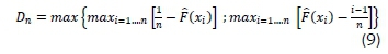
which is the largest vertical difference between the theoretical and empirical CDF for all values of χ (Evans et al., 2008), where η is the sample size.

The Anderson Darling test is also a statistical test of whether a given sample of data is drawn from a given probability distribution. It is a modification of the Kolmogorov-Smirnov test and gives more weight to the tails of a statistical distribution than that test. In its basic form, the test does not assume a particular parametric form of the distribution being tested, in which case the test and its set of critical values is distribution free. The test is, however, most often used in context where a family of distributions is being tested, in which case the parameters of that family need to be estimated and account must be taken of this in adjusting either the test-statistic or its critical values. When applied to testing if a normal distribution adequately describes a set of data, it is one of the most powerful statistical tools for detecting most departures from normality.

The test assesses whether a sample comes from a specified distribution. It compares the observed CDF with the expected CDF and is defined in Equation 10:

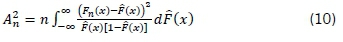
with the computational formula given by Equation 11:

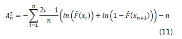
where η is the sample size. According to Abbas et al. (2012), the Anderson-Darling test is superior where there is greater concern for the extreme values in the data. This is very relevant when considering atmospheric emissions data.

The P-P and Q-Q plots are graphical methods used to test the fit of the distributions to the data. The P-P plot assesses whether or not the data set follows the specified distribution. The P-P plot compares the CDF of the distributions by plotting the theoretical values and the points of the empirical distribution against it. The Q-Q plot compares the distributions by plotting their quantiles against each other. With the Q-Q plot, the data are plotted against the theoretical distribution. For both the P-P and Q-Q plots, if the empirical distribution is close to the theoretical distribution, the graph will be a straight line (Beirlant et al., 2004). Departures from the straight line indicate the departures from the theoretical distribution.

 

4. Results and discussions

The data is from Eskom, for the period January 2005 to January 2012.The efficiency of the power station cannot be determined by absolute emissions, but by the amount of SO2 emitted in kilograms per gigawatt hours (kg/GWh) of electricity sent out (relative emissions). To accommodate the non-station-arity in the data, the total emissions of SO2 emitted (in kilograms or milligrams) per month per power station is divided by the total amount of units of power sent out per power station per month or by the volume. The derived data for the power stations, therefore, represents the amount of emission emitted in kilograms to send out one unit of power in gigawatt hours or in milligrams per cubic nano metre (mg/Nm³). The resultant variables are a measure of efficiency of the station in emitting SO2 and will be used for the analysis.

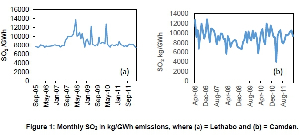
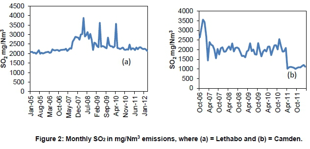
Time plots are useful for checking obvious patterns in the data. The plots represent evolving efficiency at the power stations. Time plots of Lethabo and Camden power stations' SO2 kg/GWh and SO2 mg/Nm³ data are given in Figures 1 and 2 respectively. The rest of the time plots are given in supplementary information.

Arnot, Komati, and Kriel have average monthly SO₂ emissions of around 6000 kg/GWh; Duhva, Grootvlei, Hendrina, Hendrina, Lethabo, Majuba, Matimba, Matla and Tutuka average 8000 kg/GWh; and Camden, Kandal and Matimba average emission around 9000 kg/GWh.

For SO₂ in mg/Nm³ most power stations (Cam-den, Duhva, Hendrina, Kendal, Lethabo, Majuba, Matla and Tutuka) have an average monthly emission of 2000, and Arnot, Grootvlei, Komati and Kriel 1600. Graphs for Lethabo and Camden are given in Figure 2, the remainder in the supplementary information. Matimba had the highest monthly average of 3000 mg/Nm³. Matimba received the 2011 National Association of Clean Air award for consistent reduction of point source particulate emission (COPFIT Fact Sheet, Eskom, 2012), but it seems not to be the case for SO2 emissions. An augmented Dickey-Fuller test for stationarity was carried out for all of the stations for both SO2 in kg/GWh and SO2 in mg/Nm³ at 5% significance level, showing that all stations were stationary, that none of the stations had a trend.

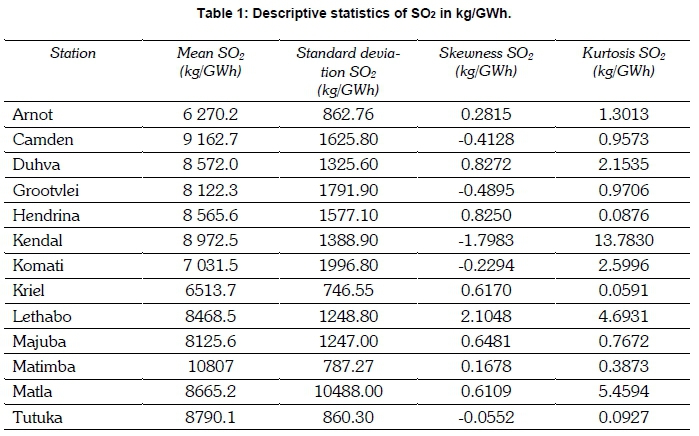
Table 1 gives the descriptive statistics of the power stations for SO2 in kg/GWh, and Table 2 gives the statistics for SO2 in mg/Nm³. Figures 3 and 4 give graphical plots of the monthly means for each station for both SO2 in kg/GWh and SO2 in mg/Nm³ from the worst to the better emitters.

 

 

 

 

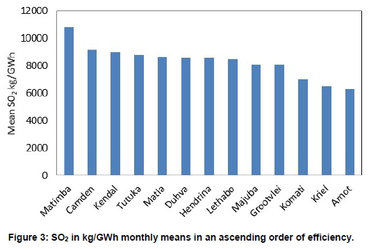
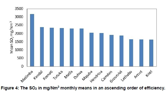
From Figures 3 and 4 it can be concluded that Matimba and Kendal are the least efficient stations in emitting SO₂, with Arnot and Kriel the most efficient.

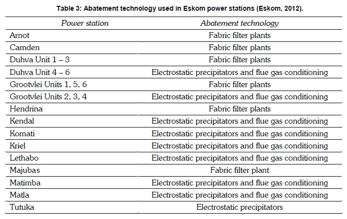
Eskom installed abatement technologies at each power station to reduce the ash emissions. These technologies are said to have an efficiency of at 99%, and over 99.9% in many cases (COPFIT Fact Sheet, Eskom, 2012). These abatement technologies are given in Table 3.

From Figures 3 and 4 in conjunction with Table 3, it can be concluded that the stations that use an electrostatic precipitators and flue gas conditioning technology are less efficient than the ones using fabric filter plants, but other factors also affect emission efficiency, including the age of the plant and the quality of coal used.

To further describe the distribution of the data we look at skewness and kurtosis of the data. The skewness is defined by Equation 12:

where μ and σ are the mean and standard deviation of emission efficiency variable x. The skewness shows how symmetric the data is around the mean. A symmetric data has skewness near zero, while negative skewness indicates that the data is spread more to the left of the mean and positive skewness indicates that the data is spread to the right of the mean. By negative-skewed, the left tail is long relative to the right tail, and by positive-skewed the right tail is long relative to the left. For SO₂ in kg/GWh, Camden, Grootvlei_a Kendal, Komati and Tutuka have a negative skewness, indicating that their data is more spread to the left of the mean. For the rest of the stations the data is more spread to the right of the mean. For SO₂ in mg/Nm³, Arnot, Grootvlei, and Matimba have a negative skew, and all the other stations have a positive skew. Only Grootvlei is confirmed with a negative skewness in both data sets.

The kurtosis is defined by Equation 13:

where μ and σ are the mean and standard deviation of χ. Kurtosis is a measure of whether the data sets are heavy- or light-tailed relative to the normal distribution. That is, data sets with high kurtosis tend to have heavy tails, or outliers. Data sets with low kur-tosis tend to have light tails, or a lack of outliers. If a distribution has a kurtosis less than three, its tail is shorter and thinner and its peak is flatter and broader than the normal distribution (Brown 2011). For SO2 in kg/GWh, only Kendal, Lethabo and Matla have a kurtosis higher than three, indicating that they have a central peak higher and sharper and that their tails are longer and fatter than that of normal distribution. All the other stations have a tail shorter and thinner and their peaks are flatter and broader than the normal distribution.

Since most stations are positively skewed for both SO2 in kg/GWh and SO2 in mg/Nm³, a right-skewed distribution needs to be considered, indicating that it could be reasonable to fit a 3LL distribution to the data. Tables 4 and 5 give the parameter estimates of the 3LL distribution for both the SO2 in kg/GWh and SO2 in mg/Nm³. The parameters are estimated using the ML estimation method.

The normal, log-normal and three-parameter Weibull distributions were also fitted to the data for comparisons. Figure 4 shows the fit to the Lethabo station, with the comparisons for the distributions.

Probability-probability and quantile-quan-tile plots: The P-P and Q-Q plots are graphical methods used to test the fit of the distributions to the data. Departures from the straight line indicates departures from the theoretical distribution. Figure 5 (split over this page and the next) gives the PDF, CDF, P-P and Q-Q plots of Lethabo station for both SO2 kg/GWh and SO2 mg/Nm³.

The PDF, CDF together with the P-P and Q-Q plots shows a better fit for the log-logistic compared to the other distributions. Looking at the Q-Q plots it can be observed that the quantiles of 3LL and the three-parameter Weibull are closer to the straight line compared to the normal and the log-normal distributions. A goodness of fit is also done on the stations. To test for the goodness of fit, the Kolmogo-rov-Smirnov and Anderson-Darling tests are considered, and the results for these are given here. The Kolmogorov-Smirnov critical value at 0.05 and 0.01 level of significance for Arnot, Duhva, Hen-drina, Kendal, Kriel, Lethabo, Majuba, Matimba, Matla and Tutuka are 0.14355 and 0.17223 respectively, and for Camden its 0.15755 and 0.18903. For Grootvlei and Komati, since their emissions were recorded from April 2009, the critical values are 0.22119 and 0.2632 respectively. The Anderson-Darling critical values at 0.05 and 0.01 significance level are 2.5018 and 3.9074 respectively. The null and alternative hypotheses are given as:

• H₀: The data follows the three-parameter log-logistic distribution.

• H_a: The data do not follow the three-parameter log-logistic distribution.

Table 6 gives the Kolmogorov-Smirnov and Anderson-Darling test results for each station.

Both the Anderson-Darling and Kolmogorov-Smirnov tests do not reject the null hypothesis for any of the stations for both SO2 kg/GWh and SO2 mg/Nm³ at 5% and 1% significance level. Supplementary information gives the QQ plots for all the other stations. Tables 7 and 8 give the probabilities of exceedances above a given threshold, where t is the threshold and P(X > t) is the probability of the exceedances.

Tables 7 and 8 show that Grootvlei, Kendal and Komati have a probability of almost zero for exceeding 5000 kg/GWh SO2 emission level per month, with Arnot, Grootvlei Majuba having a probability of almost zero for exceeding 1000 mg/Nm³ SO2 em-mission level per month. Matimba, Lethabo and Matla have a probability of 1 for exceeding 7000 kg/GWh SO2 emmission level per month with Matla, Tutuka and Duhva have a probability of 1 for exceeding 2000 mg/Nm³ SO2 emmissions per month. This confirms that the least efficient stations with regard to emission of SO2 are Matimba, Lethabo and Matla.

 

Conclusions

Monthly SO2 emissions in kg/GWh and in mg/Nm³ have been considered for Eskom's 13 coal-fired power-generating stations. The 3LL fits the data of these stations best, and makes it is possible to quantify (in terms of a statistical distribution). This quantification helps to monitor and manage the SO2 emissions effectively.

The parameters of the log-logistic distribution are estimated by the ML method. Kolmogorov-Smirnov and Anderson-Darling tests are used to test for the goodness of fit of the 3LL distribution for the 13 stations. The PDF, CDF, P-P and Q-Q plots are used to show how well the distribution fits the data.

Considering Figures 3 and 4 together with Table 4, it can be concluded that the stations that use electrostatic precipitators and flue gas conditioning technology are less efficient than those using fabric filter plants technology, although other factors, such as the age of the plant and the quality of coal used affect emission efficiency.

Tables 7 and 8 show Arnot, Grootvlei and Kriel as the most efficient stations and Matimba, Lethabo and Matla as the least efficient. Looking at the results of the goodness fit, at both 5% and 1%, the null hypothesis for all stations for both the SO2 in kg/GWh and in mg/Nm³ cannot be rejected and it is therefore concluded that the data follows the 3LL distribution. The calculated probabilities can be used to estimate costs of exceeding the given limits.

The goodness of fit tests considered show that the 3LL fits the data of the Duhva, Hendrina, Ken-dal, Komati, Kriel, Lethabo and Matimba better than other stations. For SO2 in mg/Nm³, the three-parameter log-logistic fits the data of Camden, Duhva, Hendrina, Komati, Kriel, and Lethabo best. From the results it shows that three-parameter log-logistic fits the positively skewed data better than the negatively skewed data. For the negatively skewed stations, it is only the three-parameter Weibull distribution that does better than the 3LL distribution. The three-parameter Weibull distribution is very close to the 3LL distribution in terms of goodness of fit. In emissions monitoring, however, concerns are more with high emissions (positively skewed), which give rise to undesirable consequences.

Reporting on environmental performance has several benefits, including providing management information to help exploit the cost savings that good environmental performance usually brings and, giving Eskom the opportunity to set out what they believe is significant in their environmental performance.

Further research will be done on the other Burr-type distributions to see if they will fit the data of most stations similar or better than the 3LL. The impact of the age of the plant and the quality of the coal used on atmospheric emission efficiency also requires research.

 

Acknowledgement

The authors are grateful to Eskom for providing the necessary data that made this research possible. Opinions expressed and conclusions arrived at are those of the authors and are not necessarily to be attributed to Eskom.

 

References

Abbas, K.; Alamgir.; Khan, S.A.; Ali, A.; Khan, D.M.; Khalil, U. 2012. Statistical analysis of wind speed data in Pakistan. World Applied Sciences Journal 18(11): 1533-1539.         [ Links ]

Ashkar, F. and Mahdi, S. 2003. Comparison of two fitting methods for log-logistic. Water Resources Research 39(8): SWC 7.1-SWC 7.8        [ Links ]

Balakrishnan, N. and Malik, H.J. 1987. Best linear unbiased estimation of the location and scale parameters of the log-logistic distribution. Communication in statistics A: Theory and Methods 16: 3477-95.         [ Links ]

Beirlant, J., Goegebeur, Y., Teugels J., De Waal, D. and Ferro C. 2004. Statistics of extremes. West Sussex: John Willey & Sons.         [ Links ]

Brown, S. 2011. Measures of shape: Skewness and kurtosis. Available online at: http://web.ipac.caltec.edu/staff/fmasci/home/statistics_refs/SkewStatSig-nif.pdf.         [ Links ]

Burr, I. 1942. Cumulative frequency functions. Annals of Mathematical Statistics. 13(2): 215-232.         [ Links ]

Eskom. 2011. Eskom emission monitoring. Available online at: http://www.wonderware.co.za/content/Eskom%20Emission%20Monitoring.pdf.         [ Links ]

Eskom. 2012. Kusile and Medupi coal-fired power stations under construction. Available online at: http://www.eskom.co.za/OurCompany/Sustainable-Development/ClimateChangeCOP17/Docu-ments/Kusile_and_Medupi_coal-fired_power_stations_under_construction.pdf.         [ Links ]

Eskom. 2012. Climate change COP 17 fact sheet. Available online at: http://www.eskom.co.za/OurCom-pany/SustainableDevelopment/ClimateChan-geCOP17/Documents/Air_quality_and_climate_change.pdf.         [ Links ]

Evans, D.L., Drew, J.H. and Leemis, L.M. 2008. The distribution of the Kolmogorov-Smirnov, Cramervon Mises and Anderson-Darling tests statistics for exceptional populations with estimated parameters. Communication in Statistics-Simulation and Computation 37: 1396-1421.         [ Links ]

Georgopoulos, G.P. and Seinfeld H.J. 1982. Statistical distributions of air pollutant concentrations. Environmental Science and Technology 16(7): 401A-416A.         [ Links ]

Hadley, A. and Toumi, R. 2003. Assessing changes to the probability distribution of sulphur dioxide in the UK using lognormal model. Atmospheric Environment 37: 1461-1474.         [ Links ]

Mielke, P.W., & Johnson, E.S. 1973. Three parameter Kappa distribution maximum likelihood estimates and likelihood ratio tests. Monthly Weather Review 101, 701-709.         [ Links ]

Mitchell, B. 1971. A comparison of Chi Square and Kol-mogorov-Smirnov tests. Area 3(4): 237-241. Available online at: https://www.jstor.org/stable/20000590?seq=1#fndtn-page_scan_tab_contents        [ Links ]

Rumburg, B., Alldredge, R. and Claiborn, C. 2001. Statistical distributions of particulate matter and error associated with sampling frequency. Atmospheric Environment 35: 2907-20.         [ Links ]

Seifeld, J.H. and Pandis, S.N., 1998. Atmospheric chemistry and physics: From air pollution to climate change. New York: Wiley.         [ Links ]

Singh, V.P., Gou, H. and Yu, F.X., 1993. Parameter estimation for 3-parameter log-logistic distribution (LLD3) by Pome. Stochastic Hydrology and Hydraulics 7: 163-177.         [ Links ]

Smith, L.R. 1989. Extreme value analysis of environmental time series: An application to trend detection in ground-level ozone. Statistical Science 44: 367-393.         [ Links ]

Tiku, M.L. and Suresh, R.P. 1992. A new method of estimation for location and scale parameters. Journal of Statistical Planning and Inference 30: 281-292.         [ Links ]

Wingo, D.R. (Metrica). 1993. Maximum likelihood methods for fitting the Burr Type XII distribution to multiply (progressively) censored Life Data. 40: 203-210. doi:10.1007/BF02613681.         [ Links ]

Zaharim, A., Najid, S.K., Razali, A.M. and Sopian, K. 2009. Analysing Malaysian wind speed data using statistical distribution. Proceedings of the 4th IASME/WSEAS International Conference on Energy and Environment, Cambridge, UK.         [ Links ]

 

 

* Corresponding author: Tel: +27 (0)51 401 9697 Email: girmayme@ufs.ac.za