Modelling household electricity consumption in eThekwini municipality

 

 

Samantha Reade^*; Temesgen Zewotir Delia North

Statistics Department, School of Mathematics, Statistics and Computer Science, University of KwaZulu-Natal (Westville Campus), Private Bag X 54001, Durban 4000, South Africa

 

 

---

ABSTRACT

South African municipalities are faced with the challenges of growing demand for services. This study models the energy consumption estimation practice within the Durban municipal area. It was found that an estimation technique that accounts for the seasonal and monthly effects, as well as residential type, predicts monthly individual household electricity consumption with minimum error. Models that were developed may be used to estimate electricity consumption for household billings within a municipality.

Key words: electricity consumption, mixed models, municipalities, billing

---

 

 

1. Background

The eThekwini municipality, which includes the city of Durban, is situated on the East Coast of South Africa, within the province of KwaZulu-Natal. It covers a land area of approximately 2000 km², with a population of 3.4 million. The licensed distributor of electricity to the municipality, eThekwini Electricity supplies 655 338 households with electricity, approximately half of which are prepaid customers and half are credit customers. All credit customers have an electricity meter on their property. Ideally, credit customers are charged monthly for the amount of electricity they consumed during the previous month, but for technical and personnel reasons, electricity meter readings are taken at three-month intervals. If the data collector has no access to the meter, the reading is done in the following three-month visit, and, if again the meter is not accessible during that visit, the next reading reads for the last nine months' consumption, and so on. In the meantime, however, the household is obliged to pay the estimated consumption charges and only upon the actual reading are the estimated billings adjusted backwards, with any difference then credited or debited to the household in the following month's billing. Whenever the actual reading is available, the credit or debit accrued from the previous estimates, plus the new measured consumption for that month, will be billed. In other words, the actual consumption values are used to adjust the previous estimates and predict monthly household consumption values for the months until the next reading.

Household electricity consumption is estimated by eThekwini Electricity by means of a cumulative total of weighted previous actual usages, whereby the most recent consumptions carry the highest weightings, while weights of older consumptions decrease in a geometric progression. The method may be expressed in terms of Equation 1:

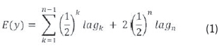
where n is the total number of actual measurements that each household has; E(y) represents the expected electricity usage, and lag_krepresents the k^th lagged actual consumption value converted per month.

The lag₁ carries a weight of 0.5, lag₂ carries a weight of 0.25, lag₃ carries a weight of 0.125 and lag₄ carries a weight of 0.0625, etc. Once these weighted lags are summed, it becomes evident that the bulk of the estimate for current electricity usage comes from the first four lags that a household has. This customary estimation method clearly does not allow for any seasonal or cyclical trends in consumption, nor does it take into account individual household electricity consumption variability and patterns.

Little research has been done, in either South Africa or other developing countries, to find models that will assist utilities to better predict monthly household electricity consumption. A primary focus of local research has been the national aggregate electricity demand and the examination of factors likely to influence it. In the 1980s, Pouris (1987) used annual data and an unconstrained distributed lag model to estimate long-run price elasticity of the aggregate electricity demand. More recently, Inglesi

(2010) specified variables that could be used to explain aggregate electricity demand in South Africa, and determined that a long-run relationship exists between electricity consumption, electricity price and economic growth. Sigauke and Chikobvu

(2011) captured the effect of various short-term demand-influencing factors such as days of the week and temperature, by developing a combination regression-SARIMA-GARCH model to predict daily peak aggregate electricity demand. Further to their 2011 study, Chikobvu & Sigauke (2013) then employed a piecewise linear regression model and applied extreme value theory to model the influence of temperature on South Africa's daily average electricity demand.

Following a model similar to that of Pouris (1987), Ziramba (2008) examined electricity demand as a function of gross domestic product (GDP) per capita and electricity price in the South African residential sector. Ziramba found that, in the long run, income was the main factor that determined residential electricity demand, while the price of electricity was insignificant. Similar studies where residential electricity demand has been modelled as a function of GDP per capita, price and other factors, have been carried out in Australia, the United States, Sri Lanka and Taiwan. In addition to studies where the focus has been price elasticity or forecasting electricity demand, research has also gone into other factors affecting electricity consumption. Firth et al. (2008) identified trends between electricity consumption and appliance usage. Marvuglia and Messineo (2012) used artificial neural networks for short-term electricity forecasting in Italy and focused on how the use of air-conditioning affected electricity consumption. Yohanis et al. (2008) carried out a comprehensive study in Northern Ireland on the patterns of electricity consumption of 27 households, taking into account a wide range of household factors such as dwelling type, location, dwelling size, household appliances, attributes of the occupants and income. They found that each factor had an impact on electricity consumption.

Aside from the small study of 27 households by Yohanis et al. (2008), the problem with studies such as those cited is that they are not able to describe electricity consumption at the level of the individual household. Though such studies are useful to estimate national residential electricity usage, the main challenge in South Africa is service delivery at the municipal and ward levels. The present study therefore initiates and motivates further research on estimating the electricity consumption of a typical household in a given municipality in South Africa. The customary practice in estimating present electricity consumption is based on prior consumptions only. Intuitively, prior consumption should serve as a good estimate for current consumption, but the challenge lies in how to best weight these prior consumption values so as to ensure accurate estimates. This study investigates how to weight prior consumption values in estimate current electricity consumption. A further aim is to ascertain whether all available lags for a household are important or not, and if there is any seasonal pattern in household consumption. The study differs from the literature cited in that the main focus is at a household level, as opposed to modelling and predicting consumption for the entire residential sector. The traditional time series and econometric modelling approaches are replaced by an applied statistical approach.

 

2. Data description

Data for this study was provided by eThekwini Electricity, from meter readings perpetually carried out at three-month intervals amongst credit customers. Meter readings, reading dates and actual consumption values are all stored on the municipality's database for combined online information systems. Other data that are stored include electrical connection identifiers, property identifiers and dwelling-type classifications. Dwellings are classified into three types: houses, share blocks that are one or two storeys high (e.g. simplex or duplex), and share blocks of more than two storeys (e.g. blocks of flats). This classification information was supplied by eThekwini Electricity, as well as meter-reading data for the five-year period 2008-2013. For this study individual electricity consumers were identified by their electrical connection identification, and are referred to as households. Additional information, such as month of meter reading and length of usage periods (defined as the time, in days, between two consecutive meter readings), was also extracted from the data provided.

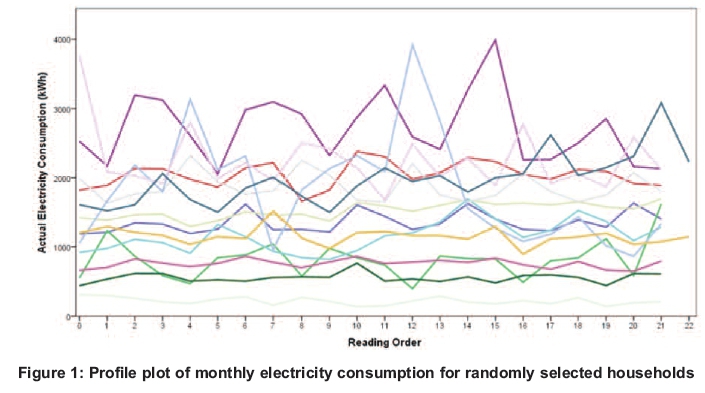
The original data set received from eThekwini Electricity was large, containing information for approximately 300 000 households, along with three-monthly consumption values for each household. Computing power required for processing such large data exceeded the available computing facilities at the University of KwaZulu-Natal, but, as the main focus was modelling electricity consumption so as to enable future prediction, using a randomly selected sample was sufficient. A sampling frame was specified so as to ensure that only households with regular meter readings at three-month intervals were considered and that each dwelling type was represented. Accordingly, a sample of 1 478 households was randomly selected from the data set. Electricity consumption was modelled for the sampled data, demonstrating effective methods that could be implemented on a larger scale (with the necessary computing capacity). A focal point of this study was to investigate the presence of a seasonal effect so as to enable better modelling of electricity usage. The starting point was, therefore, examining a simple profile plot of a few randomly selected households from the sample.

Figure 1 shows that household electricity consumption is a constant function with dominant individual variability. Moreover, this individual variability also shows some systematic cyclic seasonality, which can be accounted for by month-to-month variation. An overall seasonal pattern is, however, difficult to distinguish by simply studying the profile plot. Possible reasons for the obscured seasonality could be that there are both different dwelling types and different measurement batches that exist but are not accounted for in Figure 1. A measurement batch is a particular measurement pattern of three-month intervals that each household follows. For example, if a meter is read in January, subsequent readings will always be done in (approximately) April, July and October, then cycle back into January. As meter readings are carried out in intervals of three months, there are only three measurement batches: Batch 1: January, April, July, October; Batch 2: February, May, August, November; Batch 3: March, June, September, December. In order to better understand factors affecting monthly electricity consumption and any seasonal trends within it, the research proceeded by studying profile plots by dwelling type and measurement batch.

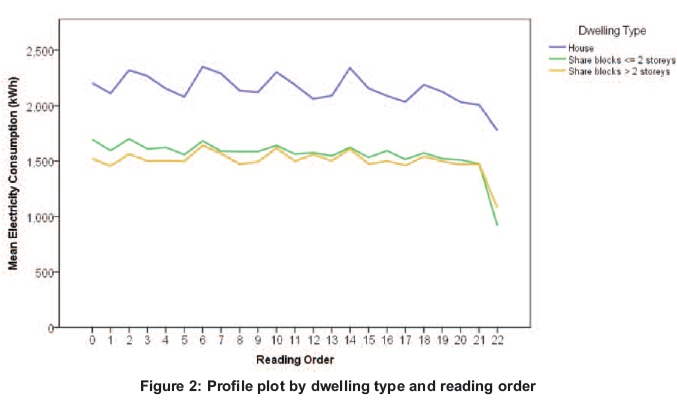
Figure 2 shows a clear difference between the consumption patterns of the three dwelling types, with houses having the highest electricity usage. Although a clearer systematic cyclical pattern in the prior consumption values is observed in Figure 2, it is still difficult to identify an overall seasonal trend, probably because, within each dwelling type, households may be further classified into the different measurement batches. Moreover, minor variations within each batch arise due to eThekwini Electricity following a measurement system of 90 days as opposed to calendar months, as well as factors such as local elections or holidays also leading meter readings to be postponed or brought forward. Although this study was most concerned to model seasonal effects within each household, and not reading-batch variability, it is acknowledged that these batch variations may cause the obscured seasonal pattern. A simple way of demonstrating this is to study the batch profiles given in Figure 3, which show the number of households and average consumption by month for the five-year period.

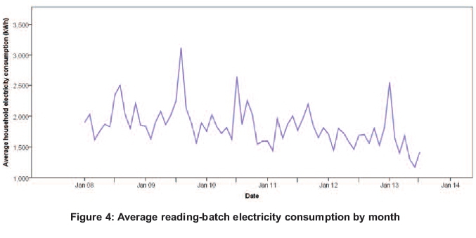
Figures 3(a) and 3(b) show that there is individual batch variability present in both the consumption values and number of households. Figure 3(a) clearly shows three distinct measurement patterns and evidence that meter-readings follow periods of more-or-less three months. Batch 3 appears to have the most number of households, followed by batch 2 and then batch 1. A possible reason for this variation could be that some batches come from more densely populated areas than others, resulting in more meter-readings. From Figure 3(b) it can be observed that, within each batch, some form of monthly effect is taking place, as some months show higher consumption values than others. An overall monthly pattern is difficult to determine in Figure 3(b), however, possibly due to each reading-batch having its actual consumption values recorded at different times. To better understand the month effect, a profile plot of the average electricity consumption of the reading-batches by month over the five-year period was examined; the plot is displayed in Figure 4.

The plot shows that higher electricity consumption values generally occur in July, August and September. Given, however, that meters are read at three-month intervals, the consumption values for the months in Figure 4 also refer to consumption values of approximately two months prior to the month of meter reading. In the 90-day interval, the 'middle' month is the month where the monthly consumption could be deduced. From this understanding it can be seen that the months of high consumption reading, July, August and September, in fact refer to an approximate median June-August period of higher electricity usage. It is necessary to be vigilant with regard to metre-reading months and actual consumption months. The reading month is given, so the inference should be the consumption pattern of two months earlier. Conscious of this, it is essential to examine the two sources of the cyclical seasonal effect. The first element is the monthly seasonal effect observed in Figure 4, whereby the winter months gave evidence of increased electricity consumption. The second possible element is autocorrelation within each household's annual electricity consumption values.

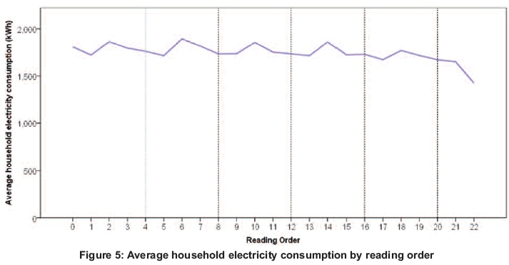
In order to further investigate the presence of autocorrelation, another profile plot was examined, this time averaged over each household by reading order, given in Figure 5. From the graph, it can be noted that some form of autoregressive process is taking place. The consumption values at t=0, 4, 8, 12 and 20 are similar. The same pattern is observed at t=2, 6, 10, 14 and 18. Since there are three months between consecutive meter-readings, after four meter readings 12 months have passed. Likewise, after eight readings, it can be assumed that 24 months have passed; after 12 readings 36 months have passed, and so on. One way to account for such an autoregressive pattern in the data is to include some lagged values in a linear model . The current study employed a linear mixed modelling approach which is well-suited to handling repeated measures and accounts for variations both between and within households. Using linear mixed models (LMMs) allows modelling of both the month-to-month seasonality as well as the repetitive pattern occurring in prior consumption values. Moreover, mixed models are flexible, allowing for the both temporal and spatial variations to be modelled.

 

3. Methodology

Laird and Ware (1982) were the first to illustrate the use of LMMs in longitudinal data analysis. Subsequently, many researchers have used both LMMs and generalised LMMs (GLMMs) to model repeated measures data. The GLMM is the generalised form of the LMM, whereby the response variable may come from a variety of distributions, provided the distribution is a member of the exponential family . The general form of a linear mixed model, adapted for repeated measures data, is given by Equation 2.

where y_i = (y_i1, y_i2, y_ini)', if y_ij represents the response of the i^thindividual measured at time t_ijfor i = 1, ... , N and j = 1, ... , n_i; Xi is an (n_i× p) matrix of known covariates associated with the fixed effects; β is a (p × 1) vector of unknown regression parameters representing the fixed effects; Z_i is an (ni × q) design matrix associated with the random effects; b_i is a (q × 1) vector of random effects, representing the random subject-specific effects, such that b_i ~ N(0, G) where G is block diagonal with the i^thblock being σ_i² I_qi; e_i is an (n_i× 1 ) vector of residual components where it is assumed e_i ~ N(0, R) and R is positive definite. Furthermore, it is assumed that b_i and e_i are independent. Different variance-covariance structures may be fitted to R, allowing us to model both spatial or temporal variance and correlation. In the GLMM, the conditional expectation of y is related to a linear predictor (η) by means of a monotonic differentiable link function g(.). The general form of such a GLMM for repeated measures data is given by Equation (3).

where η_i represents the linear predictor of the i^th individual and g(.) the link function that links the conditional mean, E(y_i|b_i) to the linear predictor.

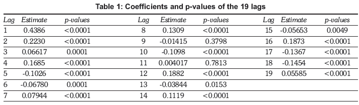
There are essentially three aspects to consider when specifying and fitting a GLMM to the electricity data: the specifications of the covariates in the model, the selection of the best suited covariance structure, and the selection of the distribution that best fits the response variable. To begin the modelling process current electricity consumption is initially assumed to be normally distributed. That is, it is first established which covariates to include and what covariance structure to fit, then a search is made for the distribution best suited for the electricity data. Having already established that dwelling type, month of meter reading and prior consumption values in some way affect current electricity usage, a marginal linear regression model is tentatively fitted, where current household electricity consumption is modelled as a function of all of these factors. As meters are read at three-month intervals, each household can be expected to have a minimum of 20 measurement occasions for the five-year period. Therefore, each household can be expected to have a minimum of 19 lagged values. To determine whether or not it is necessary to retain all 19 lags in the model, their significance and coefficient values are studied. These values are displayed in Table 1.

Table 1 shows that all the lags except for lags 9 and 11 are significant at a 5% level of significance. However, despite the significance of lags 13 to 19, upon closer examination of their coefficients it can be noted that these lags have, in fact, little overall effect on current household electricity consumption. That is, the coefficients of lags 13 to 19 contribute little, due to the positive coefficients of lags 14, 16, and 19 and the negative coefficients of lags 13, 15, 17 and 18 almost cancelling each other out. This shows that there is little value in retaining more than 12 lagged values in the regression model. Hence, in the interests of parsimony, the modelling process is continued using only 12 lags in the model, which is equivalent to a household's three-year electricity consumption cycle. In addition to the 12 lags, the month of the most recent meter reading and dwelling type in the linear model are retained. By including both lags and month of meter reading in the model, two different factors can be analysed. The inclusion of the month of meter reading enables the taking into account of months that may have higher or lower electricity consumption than others. Lags allow for the incorporation and assessment of the cyclical seasonal pattern observed within household electricity usage. Using month of reading, dwelling type and 12 lagged values, the following linear model is specified, noting that two dummy variables have been created for dwelling type and eleven dummy variables for the month of meter reading according to Equation 4.

where g(.) is the link function, E(y_ij) is the expected response of the i^thhousehold, i = 1, ... ,1478 at time j = 1,2, ... , n_i, where n_iis the number of actual readings for household i; a_i0represents a household-specific random intercept; and h_ijis the linear predictor. As the data is initially assumed to be normally distributed, a normal distribution is specified and the identity link function is used. By including a household-specific random intercept, the variability of different households within the variance components can be accounted for.

Following model specification, the next focus is on modelling within-household temporal variations. Several temporal covariance structures are fitted to the model, namely unstructured (UN), compound symmetric (CS), first-order autoregressive (AR(1)), autoregressive moving-average of order one (ARMA(1,1)), first-order ante-dependance (ANTE(1)) and Toeplitz (Toep). To determine the best-suited structure, several factors are considered: the Akaike information criteria (AIC), the number of parameters that require estimating and the convergence status of the model. Ideally, the structure selected converges successfully, has a small AIC value and only a few parameters. Amongst the fitted structures, Toep and ANTE(1) failed to converge successfully, so were discarded as viable structures. Table 2 displays the fit statistics of the structures that converged to a solution.

 

 

Table 2 shows that the unstructured model renders the smallest AIC value, but it is discounted as unviable, because it also has the highest number of parameters that require estimating. Following the unstructured form, the next best model is the ARMA(1,1) structure. Not only does this model have the second smallest AIC value, but it also has only three parameters that require estimating. The ARMA(1, 1) structure is therefore selected as the best-suited covariance structure. Having now modelled within-household temporal variation by means of selecting a covariance structure, the third and final aspect of specifying a GLMM for the electricity data is undertaken: searching for the distribution most appropriate for the electricity data. To do so, a variety of link functions are considered, and five distributions that belong to the exponential family, namely the normal, namma, lognormal, inverse Gaussian and exponential distributions. Only two converged to solutions: the normal distribution (AIC=184306.1) and the Lognormal distribution (AIC=3815.57), both with the identity link. However, according to the smaller-is-better Akaike information criteria, the lognormal distribution is clearly to be favoured over the normal distribution. Further support for choosing the lognormal distribution is that it is a distribution that naturally only takes non-negative values, making it compatible with electricity consumption data which can also only take on non-negative values. Nevertheless, despite the compatibility of the lognormal distribution, it is still necessary and important to assess the goodness of the underlying distribution assumptions. To do so, both the scatter and probability plots of the conditional studentised residuals are examined (Zewotir and Galpin, 2004). These plots are depicted in Figures 6 and 7(a).

 

 

For the majority of cases in the scatter plot of Figure 6, an evident random scattering about zero is obvious. This supports the non-existence of any systematic pattern not accounted for by the model. It is also noteworthy, however, that several cases drift away from zero but, given that such cases are few in relation to the large data, these points can be classified as outliers. From the Q-Q plot in Figure 7(a), it is clear that most of the points lie approximately on the straight line, favouring the goodness of the lognormal distribution. The tails that depart from the line are due to a few outlying households in the data. Based on the plots in Figures 6 and 7(a), it can be comfortably concluded that both the distributional and linearity assumptions have been adequately satisfied, except for a few outliers. In repeated measures data analysis it is necessary to ascertain whether or not outlying subjects are influencing the model fit and, more specifically, if they are exhibiting influence in the covariance parameter estimates (see Zewotir & Galpin, 2006; Zewotir , 2008). If an outlying subject is identified as being influential it should be removed from the data, and any inferences ought to be based on the reduced-data model. Such identified subjects must, however, undergo scrutiny in order to determine any case anomalies. The case outliers in Figures 6 and 7(a) belong to households 202 and 1205, and their effect can be examined by running the full-data model and comparing it to subsequent reduced-data models. Influence is measured by the amount of change in covariance parameter estimates, as well as the observed effect on the AIC values and reduced-data Q-Q plots. Both the reduced and full data probability plots are shown in Figure 7, along with the AIC values.

Figure 7 shows that the individual removal of households 202 and 1205 and the simultaneous removal of both result in smaller AIC values. Although suggesting an improved model fit, this alone does not suggest influence, as a reduction in AIC values could be expected when outliers are removed. It is therefore necessary to examine the Q-Q plots and change in covariance parameters. From the near-identical plots in Figures 7(a) and 7(c), it is clear that household 1205 is not effecting influence, as little change is observed upon its removal. Figures 7(b) and 7(d) show that the removal of household 202 results in more model outliers, showing this household is better left in the model. Final evidence of the lack of effect that the removal of these outlying households have is found in the resulting covariance parameter estimates. From the tables within Figure 6, upon removal of households 202 and 1205, it is clear that there are only negligible changes in the covariance parameter estimates. The lack of significant differences in the parameter estimates, as well as the evidence portrayed in the Q-Q plots, shows conclusively that households 202 and 1205 are not influential and are merely model outliers. The data reveal a possible reason for them showing up as outliers: both have consecutive usage periods where electricity consumption is very low, compared to the majority of consumption values in other usage periods for the same households. Having confirmed that households 202 and 1205 are non-influential outliers, they are retained in the model. The conclusion is that, when considering temporal variations within the electricity data, a full-data GLMM fitted to the lognormal distribution that uses an ARMA(1,1) covariance structure and includes a household-specific random intercept is the best-suited model.

Before proceeding with model inference and predictions, however, it should be noted that the current GLMM does not take into account that the number of days in each measurement period varies slightly. Despite carefully selecting the sample data to ensure approximately evenly spaced measurement occasions, a small amount of variation is inevitable. While the variation is negligible enough to still use methods for evenly spaced data, the small variations may result in the parameter estimates no longer being efficient. A possible solution to this problem is to add weights to the estimation procedure. Accordingly, previous estimates are weighted by the length of time (in days) of an approximate monthly measurement period. Upon adding weights, an improved model fit is observed, by which the AIC value was reduced from 3815.57 in the unweighted model to 3781.15 in the weighted model. The weighted GLMM is therefore taken as the final model from which to make inferences.

 

4. Results

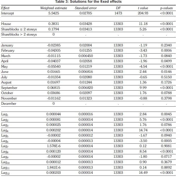
The main inferences are derived from studying the parameter estimates of the fixed effects. The type III test results for the null hypotheses show that, at a 5% level of significance, both hypotheses will be rejected, as both tests render p-values smaller than 0.0001. This indicates that at least one dwelling type and one month are significant to the model and that their individual estimates should be examined along with the lags. All fixed effect estimates are displayed in Table 3.

The first observation to be made from Table 3 is the size and significance of the model intercept, which indicates that not only is a starting value universal to all households necessary but also shows how a household-specific random intercept is likely to improve the model's prediction capabilities for individual households. Next, the estimates for the various dwelling type classifications are examined. Using share-blocks of not more than two storeys as the reference category, it is shown that houses have a parameter estimate of 0.3831 while such share-blocks have a smaller parameter estimate of 0.1794. This agrees with what was first observed in Figure 2, distinctly showing that, of the three possible dwelling types, households falling under the classification of 'house' have a higher electricity consumption than those under the classification of 'share blocks of not more storeys', provided the reference category remains the same.

The parameter estimates for the months that meters are read in are examined next. Table 3 shows that February, April, May, June and September are significant at a 5% level of significance. Of these months, relative to December, the months May and September are highly significant (having p-values of <0.0001) in the model. Of all the months, September has the highest positive parameter estimate of 0.06815, while May has the highest negative coefficient of -0.05540. This suggests that September is likely to see a rise in electricity consumption, while May is likely to see a decrease, compared to the reference month, December. The meter-reading procedure of three-month intervals and the concept of electricity consumption for a median month (referring to an approximate midpoint between consecutive meter readings) is invoked, to give an understanding that, for May and the two months preceding it, the median month would be April, while for September and two months preceding it the median month would be August. It can be deduced that median month April will likely see a decrease in electricity usage, while median month August will likely see higher electricity consumption. However, this inference depends on the reference month (December) remaining the same and on the concept of a median month being approximate, as it depends on where in the month meters are read. Increased electricity consumption in August agrees with the original observation from Figure 4 that winter months are periods of higher electricity consumption. The model provided further insight into this aspect of the seasonality by also showing periods of lower consumption.

The last of the fixed effect estimates examined are those of the lags. Table 3 shows that lags 1, 2, 4, 6, 8 and 12 are all significant at a 5% level of significance. Of these lags, however, 1, 2, 4, 8 and 12 have the largest coefficient estimates. The fact that lags 1 and 2 have high estimates indicates that the two most recent consumption values are important. The large coefficients of lags 4, 8 and 12 show that a cyclical seasonal effect is present, as they correspond respectively to 12, 24 and 36 months prior to current electricity consumption. Thus, by including lags in the linear model this aspect of the seasonal pattern can be accounted for. Following the fixed effects, the covariance parameter estimates are briefly examined, recalling that to model temporal variance an ARMA(1,1) structure was fitted, and, to enable better prediction for individual properties, a random household-specific intercept was included. The estimates are displayed in Table 4.

 

 

From the ARMA(1,1) structure it can be seen that lag₁ correlation is constant, with the corresponding covariance function being estimated by (0.2607) + (2.3799)(0.5306), where the household-specific intercept is accounted for by 0.2607. Subsequent (lag₂ and onwards) correlations decrease with the amount of time that passes between measurement occasions; that is, the covariance becomes a function of the lag and is estimated by (0.2607) + (2.3799)(0.5306)(0.6506)^lag.

 

5. Conclusion

This study used generalised linear mixed models to model electricity consumption of a typical household in eThekwini municipality. The Lognormal distribution was found to be best suited to model the electricity data and an ARMA(1,1) model was well suited to modelling within-household temporal variability. A key interest in this study was to investigate the presence of a seasonal effect in household electricity consumption. Initial data exploration suggested some form of seasonality was present, but it was difficult to distinguish. Further scrutiny of a variety of time plots suggested that there were two elements to the observed cyclical seasonal pattern: a monthly effect and a 12-month form of autocorrelation. To account for both aspects of the seasonality the most recent month of meter reading and 12 prior consumption values in the linear model were included. The inclusion of 12 prior values equated to including a household's three-year cycle of electricity consumption values. Dwelling type and a household-specific random intercept were also included in the linear model. The addition of a household-specific intercept improved the model's overall predictive capabilities, as it allowed for the capturing of some of the between-household variability.

To illustrate the effectiveness of the fitted model, predictions made using both the weighted GLMM and customary eThekwini Electricity estimation method were compared to actual monthly values. For the comparison 50 households were randomly selected and the most recent electricity consumption value that each selected household had from the data was removed, which became a desired value to predict for. Predictions were then made using both prediction methods, and to show which predictions were closest to actual monthly values, a spider graph was constructed (Figure 8), showing the absolute value of the relative errors as a percentage, for both the weighted GLMM and customary eThekwini Electricity method.

 

 

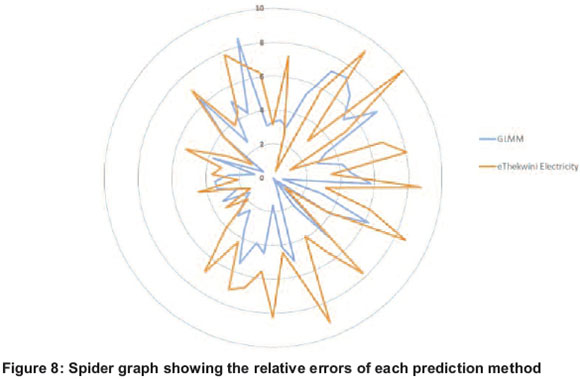
In Figure 8, the absolute value of the errors are represented by concentric circles, with the innermost circle representing the smallest error and the others showing increasingly large errors. The graph shows the weighted GLMM to be the method most closely centred in and around the inner circles, indicating that the GLMM is the better performing model, having the smallest errors across the selected households. This means that the GLMM has predictions that are close to the actual monthly consumption values for most households. The municipality's method results in the overall highest errors between predicted and observed values.

Two key findings of this study established a seasonal pattern in the prior consumption values and determined that winter is likely to see a rise in household electricity consumption. The pattern showed that, when modelling current electricity usage, a household's two most recent consumption values, and values 12, 24 and 36 months prior to the current value, are of particular importance out of all the prior values a household has, contributing the most to the prediction. This finding differs from that of the customary estimation method, in which the four most recent consumption values contribute most to the estimate. The model developed in this study provides insight into household consumption patterns as well as serving as the foundation for further studies on modelling and predicting electricity consumption at a household level. Further studies are required to find models that can adapt to less than ideal measurement circumstances that occur in the meter reading process, such as exceedingly long or unevenly spaced usage periods.

 

References

Athukorala, P. and Wilson, C. 2010. Estimating short and long-term residential demand for electrcity: New evidence from Sri Lanka. Energy Economics 32:34-40.         [ Links ]

Chatfield, C. 2004. The analysis of time series: An introduction. 6th ed. Boca Raton, Florida, USA: Chapman & Hall/CRC.         [ Links ]

Chikobvu, D. and Sigauke, C. 2013. Modelling influence of temperature on daily peak electricty demand in South Africa. Journal of Energy in Southern Africa 24(4): 63-70.         [ Links ]

Dergiades, T. and Tsoulfidis, L. 2008. Estimating residential demand for electricity in the United States. Energy Economics 30: 2722-2730.         [ Links ]

eThekwini Electricity. 2013. 2011/2012 Annual Report. Available: www.durban.gov.za.         [ Links ]

Firth, S., Lomas, K., Wright, A., and Wall, R. 2008. Identifying trends in the use of domestic appliances from household electricity consumption measurements. Energy and Buildings 40:926-936.         [ Links ]

Holtedahl, P & Joutz, F 2004. Residential electricity demand in Taiwan. Energy Economics 26:201-224.         [ Links ]

Inglesi, R. 2010. Aggregate electricity demand in South Africa: Conditional forecasts to 2030. Applied Energy 87:197-204.         [ Links ]

Laird, N. M. and Ware, J. H. 1982. Random effects models for ongitudinal data. Biometrics 38:963-974.         [ Links ]

Marvuglia, A. and Messineo, A. 2012. Using recurrent artificial neural networks to forecast household electricty consumtion. Energy Procedia 14:45-55.         [ Links ]

Narayan, P and Smyth, R. 2005. The residential demand for electricity in Australia: An application of the bounds testing approach to cointegration. Energy Policy 33:467-474.         [ Links ]

Nelder, J. and Wedderburn, R. 1972. Generalized linear models. Journal of the Royal Statistical Society Series A (General) 135 (3):370-384.         [ Links ]

Pouris, A. 1987. The price elasticity of electricity demand in South Africa. Applied Economics 19:1269-1277.         [ Links ]

Sigauke, C. and Chikobvu, D. 2011. Prediction of daily peak electricity demand in South Africa using volatility forecasting models. Energy Economics 33: 882-888.         [ Links ]

Yohanis, Y., Mondol, J., Wright, A. and Norton, B. 2008. Real-life energy use in the UK: How occupancy and dwelling characteristics affect domestic electricity use. Energy and Buildings 40:1053-1059.         [ Links ]

Zewotir, T. (2008). Infinitesimal model perturbation influence in the linear mixed model. South African Statistical Journal, 41(2), 105-126.         [ Links ]

Zewotir, T. and Galpin, J. (2004). The Behaviour of Normality Under Non-normality for Mixed Models. South African Statistical Journal, 38, 115-138.         [ Links ]

Zewotir, T. and Galpin, J. (2006). Evalution of linear mixed model case deletion diagnostic tools by Monte Carlo simulation. Communications in Statistics-Simulation and Computation, 35(3), 645-682.         [ Links ]

Ziramba, E. (2008). The demand for residential electricity in South Africa. Energy Policy, 36, 3460-3466.         [ Links ]

 

 

* Corresponding author: Tel: +27 (0)31 260 3011; email: 208506871@stu.ukzn.ac.za