RESEARCH ARTICLES

 

Evaluation of the impact of distributed synchronous generation on the stochastic estimation of financial costs of voltage sags

 

 

N. Mbuli^{I, II}; R. Xezile^{I, II}; J.H.C. Pretorius^{I, *}; P. Sowa^III

^IDepartment of Electrical, Electronic and Computer Engineering, University of Johannesburg, South Africa
^IIEskom Holdings SoC Limited, Gauteng, South Africa
^IIISilesian University of Technology, Instytut Elektroenergetyki i Sterowania, Gliwice, Polan

 

 

---

ABSTRACT

Power system faults can cause voltage sags that, if they are less than voltage sensitivity threshold of equipment, can lead to interruption of supply and lead to incurring of financial losses. The impact of distributed generation (DG) on these financial losses is investigated in this work. Using the method of fault positions, a stochastic approach to determine voltage sag performance, profiles of magnitudes of remaining voltages at a monitoring point for faults occurring along lines in the network is developed. It follows that an expected number of critical voltage sags at a monitoring point is calculated and the expected cost of these sags is derived for various voltage sensitivity threshold limits. An illustrative study is carried out comparing the expected costs of voltage sags for a network without DG with a DG case, for various mixes of customers. It is shown that in the presence of DG, the expected costs of voltage sags are lesser for all voltage sensitivity criteria assumed and for all customer mixes. The study demonstrates that the impact of incorporating DG sources results in a reduction in the expected cost of voltage sags.

Keywords: financial costs, stochastic estimation, uniform probability density function

---

 

 

1. Introduction

A voltage sag is defined in the IEEE Standard 11591995 as (Bollen, 2000) as the reduction in root mean square (rms) voltages to a value that lies between 0.1 and 0.9 for durations in the range of 0.5 cycles and one minute. One major cause of voltage sags is the faults that occur in the transmission and distribution system, leading to short circuits. Another cause is that of large currents that result when large motors are started or when transformers are energized.

Together with interruptions, voltage sags are the power quality problem that accounts for most interruption of supply to customers. Despite voltage not being reduced to zero during a sag, the voltage can be significantly lower than normal values. Thus large industrial and commercial customers who own and operate voltage voltage-sensitive equipment, such as Information Technology (IT) and process control equipment, motors, and variable speed drives can experience interruptions due to voltage sags (Dugan et al., 1996). The consequences of this are significant economic losses to the customer due to loss of production, idled labour, and other ancillary costs, such as, those related to damaged equipment and penalties due for late delivery of products.

In the recent past, a major resurgence (Ipinnimo et al., 2013) of distributed generation (DG) has been taking place. Some of the drivers for this are the initiatives aimed at reducing the global footprint of carbon dioxide emissions in order to counter global warming. In developing countries, in which resources for building large and centralized generation plants are scarce, DG presented itself as a viable alternative. Subsequently, DG offers modularity in its implementation and projects can be speedily implemented.

Numerous studies reporting the impacts of DG on voltage sags were conducted involving the impact assessment of transmission and distribution faults on voltage sags experienced by a sensitive load connected at low voltage (Ramos et al, 2014), the locations and the number of DG units on voltage sags (Rojas et al., 2013), as well as of system short circuit level, rated output of DG and model of generator (Ramos et al., 2009) used are evaluated. The impact of penetration levels is discussed in (Garcia-Martinez & Espinosa-Juârez, 2008) and the results into the study of various types (i.e., converter-connected, asynchronous and synchronous) of DG units (Renders et al., 2008) connected to the low voltage network are presented.

Some studies into the economic aspects of voltage sags were undertaken. Economic models for expressing the benefits of distributed generation were developed in Gil & Joos (2008). An approach for simultaneous reconfiguration of the network and placement of DG to reduce impact of voltage sags, while minimizing active power losses and associated financial costs, is presented in Nodushan et al. (2013). The economic benefits of commissioning DG to meet load demand is met was compared with the alternative of installing a large, centralized power station in Akorede et al. (2010).

A probabilistic methodology for calculating expected annual financial losses due to voltage sags and interruptions was developed in Milanovic & Gupta (2006). This methodology was implemented in Milanovic & Gupta (2006) in a study to compare expected annual costs of voltage sags for various topologies of distribution networks. The methodology was again used by Patne and Tharke (2010) to compare the impacts of various transformer winding arrangements on financial losses of a distribution customer due voltage sags resulting from faults in the transmission system.

Here, the results of a study into the impact of DG on the expected cost of voltage sags are presented. The voltage sag performance of the power system was determined by using stochastic method of fault positions. From this, the expected number of critical voltage sags was determined. The last step was to calculate the expected cost of voltage sags for various customer mixes and compare the values for case without DG and with DG.

The remainder of the paper is arranged as follows. The impact of distributed generation on voltage sags is discussed in Section II. The approach for calculating the expected financial losses with and without DG is discussed in Section III. In Section VI, the approach for the case study done is discussed. The results and discussions are presented in Section V. Finally, conclusions are drawn in Section VI.

 

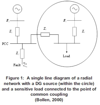
2. Analysis of voltage sags in the presence of distributed generation

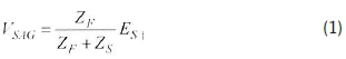
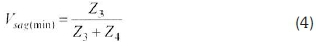
A radial power system with a DG source (encircled) and a sensitive load, both connected at the point of common coupling, is shown in Figure 1. In the absence of the DG source, if a fault occurred at the location shown, the voltage sag experienced by the customer would be the voltage at the point of common coupling (PCC). By applying the voltage divider rule (Hambley, 2014), this voltage, V_SAG, can be expressed in terms of the impedance between the source and PCC, Z_s, and the impedance between the fault and the PCC, Z_f, as

 

 

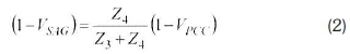
In the presence of a local generator, the voltage at its terminals during a voltage sag can be related to the voltage at the point of common coupling by

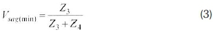
The improvement in voltage level can also be inferred from the fact that even if the voltage at the PCC dropped to zero (0), the magnitude of the voltage sag at the customer, V_sag (_mi„), could be expressed by equation (3) and is never zero (0).

Thus, in addition to (Bollen, 2000) increasing short circuit strength of networks, thereby helping to decrease the severity of voltage sags, the DG also maintains voltages during faults by feeding into faults, consequently ameliorating voltage sags.

 

3. Stochastic estimation of the economic impact of distributed generation on voltage sags

In this section, an approach for estimating the expected costs of voltage sags is presented. First, a stochastic approach to estimate voltage sag performance, using method of fault positions, is presented. Then a method of determining the number of critical voltage sags is discussed and ultimately. for estimating the cost of voltage sags is presented.

3.1 Voltage sags at a monitoring point

To determine system performance, monitoring, involving recordings, is a direct way that can be used (Bollen, 2000). The main disadvantage of monitoring is that it requires long periods of measurement. As an alternative to this approach, stochastic prediction methods for estimating the number of voltage sags were proposed, with the advantage that information was generated instantly and prediction of voltage sag performance of future networks, for which data does not exist, was made (Bollen, 2000; Juarez & Hernandez, 2006).

One of these widely used stochastic methods for predicting voltage sag performance is the fault positioning method (Thasananutariya & Chatratana, 2005; Bollen et al., 1996). It is based on assuming fault positions distributed throughout the network, with each position representing a location of faults in a particular part of a network. An illustration of this is made in Figure 2 where a transmission line between busses p and q is shown, with a possibility of a fault to occur at some location i.

 

 

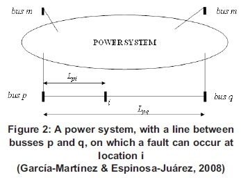
A parameter, Ψ, is used to describe the location of a fault at position i along the transmission line, i.e., to determine whether the fault has occurred at the beginning of the line (0) or at some location along the line or at the end of the line (1). Thus, this parameter may be expressed as

with L_pirepresenting the fault position i from bus p and L_pqbeing the total length of the line.

Now, suppose there is a customer location m at which voltage sag performance is to be monitored (i.e., monitoring location). To illustrate this, Figure 3 depicts the function V^a_m(Ψ), i.e., how the magnitude of remaining voltage on the faulted phase at monitoring point varies with fault position, i, on line p-q.

 

 

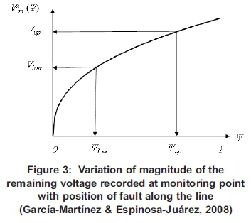
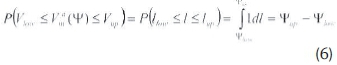
The graph shows that the probability of having a voltage sag at m with a magnitude of remaining voltage between V_lowand V_upis equivalent to the probability of having a fault between locations Ψ_low and Ψ_ιιρ. This can be expressed as

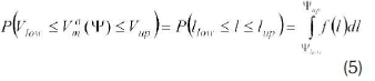
where P(V_low< V < V_up) is the probability that the magnitude of the voltage sag at point m lies between V_hw and Vup, Ρ(Ψl_ow< Ψ < Ψ up) is the probability that a fault occurs between Ψl_owand Ψ_ηρ, and f(l) is the probability distribution function of faults, with V and l in per unit.

3.2 Number of critical voltage sags

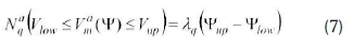
If a uniform probability density function were assumed for faults occurring in this system, equation (5) can be re-written (Wackerly et al., 2008) as

The expected number of voltage faults/annum, λ_qfor a network can be obtained from historical performance data for a particular power system. This can then be used to calculate the number, of voltage sags at a node m with the magnitudes in the V_lowto V_up, i.e. N^a_q, can be expressed using the equation

Finally, the number of critical voltage sags at node m, i.e., those that results in equipment trips, can be calculated by considering the sensitivity of equipment connected at node m, i.e., the number of critical voltage sags is the total of all those that have magnitudes that are less than the voltage threshold sensitivity of the connected equipment. The sensitivity of equipment to voltage sags is determined by using the voltage-tolerance performance curves, where the Computer Business Equipment Manufacturers Association (CBEMA) and Information Technology Industry Council (ITIC) curves (Ipinnimo et al., 2013) are widely used.

3.3 Estimation of the cost of voltage sags

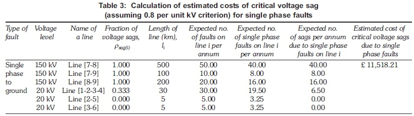
The approach for calculating the estimated cost of voltage sags is illustrated in Table 3. Here, the assumed criterion for the occurrrence of voltage sag is 0.8 per unit kV. The number of critical voltage sags at bus 1 due to single phase to ground faults, in this illustration, in the system can be calculated by using equation (8)

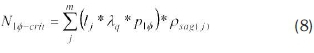
where

Ν1_Ф-crit is the number of critical voltage sags recorded at bus 1

lj is the length of line j

m is the number of lines in the system

X_qis the number of faults/km/annum for the network

Ρΐφ is the fraction of single phase to ground faults, translating to the probability of such faults

Psctg(j) is the probability of a voltage sag at bus 1 due to a fault on line i.

Once the number of critical voltage sags is determined, the estimated cost of voltage sags due single phase to ground faults can be established by using equation (9):

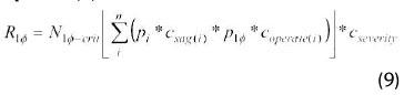
where

R₁Ф is the cost of voltage sags/annum of customers connected to a monitoring point of interest due to critical voltage sags caused by faults in the power system

N_cris the number of critical voltage sagas recorded at monitoring point due to faults in the power system

p_i is the percentage of load that is of type i (industrial, commercial, residential, etc.)

Csctg(1) is the estimated cost per voltage sag for customer of type i

c_operctte(_i) is the correction factor for duration of oper ation, representing fraction of time that customer type i is running its operations

c_severity is the scaling factor for severity of voltage sag, with a very low scaling factor for less severe sags

The above calculation is then repeated for phase to phase, phase to phase to ground faults, and for three phase faults. Finally, total estimated cost of voltage sags are obtained by adding the estimated costs for each of the four fault types.

 

4. Illustrative case study

This section provides the details of the illustrative case study done to assess the impact of distributed generation on the economic consequences of voltage sags. In this case study, transient stability studies are used to create faults at various locations along the lines, and voltage sags at some monitoring point are recorded.

The Power System Simulator for Engineering (PSS/E) (PSS/E, 2009) software is utilized in the case study. The software consists of well-established programs for running loadflow analyses and transient stability studies. The main steps in the approach of creating voltage sags are summarized as follows:

• Create a loadflow model of the network.

• Incorporate dynamic models of machines and controller, ensuring that all models initialize correctly.

• Run the system model without applying any disturbance to, for instance, 1 second to ensure that the model is stable.

• Apply a fault at a particular location in some line to initiate a disturbance in the system. For this case study, four types of faults are studied (i.e., single phase to ground, phase to phase, phase to phase to ground, and three phase faults). The duration of the fault used is 0.05 second.

• Record the voltage at the monitoring point (bus 1).

• Repeat the studies for every line starting end and every 5% of length.

• Studies are done for case with and without DG.

The single line diagram of the network used is shown in Figure 4. Faults are applied along the lines in the network and voltage sags are measured at bus 1.

 

 

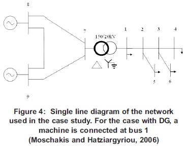
The details of data used are summarized as follows:

• Lines at 150 kV. The positive (and negative) sequence impedance is 0.097 + j0.39 Ω per unit/km. The line charging is 0.010000 S per unit /km. The zero sequence impedance is 0.497 + j2.349 Ω per unit/km.

• Lines 1-2, 2-3, and 3-4 at 20 kV. The length used for these lines is 10 km. These lines have the following parameters: (I) positive (and negative) sequence impedance is 0.22+j0.37 Ω per unit/km, (II) line charging is 0.003000 S per unit /km, and (III). The zero sequence impedance is 0.37+j1.56 Ω per unit/km.

• Lines 2-5 and 3-6 at 20 kV. Both have lengths of 10 km. Their positive (and negative) sequence impedance is 1.26+j0.42 Ω per unit/km, their line charging is 0.001000 S per unit /km, and their zero sequence impedance is 1.37+j1.067 Ω per unit/km.

• All loads have the size of 1.07 MW + j0.1 MVAr. Generator at bus 9 generates 3 MW + j3.8 MVAr, with the rest of the generation requirements provided by machine at bus 8, which is at the system swing bus.

In the case where DG is incorporated in the system, the steam turbine generator is assumed, for which a PSS/E model GENROU is utilized and the exciter model IEEET2 is used.

The rates of fault occurrence used in calculating the number of faults on 20 kV and 150 kV lines are (Patne & Tharke, 2010) one (1) and 0.1 fault/km/annum, respectively. In addition, the probabilities of occurrence of various fault types, for the two voltage levels, are as follows. For 150 kV level the probabilities are 0.8 for phase to ground faults, 0.07 for 3 phase to ground faults, 0.07 for phase to phase to ground faults, and 0.06 for phase to phase faults. In the case of 20 kV level, the corresponding probabilities are 0.65, 0.17, 0.08, and 0.1.

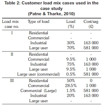
Different customer will suffer different costs in their operations due to voltage sags. The costs per voltage sag assumed in the study for various types of customers are as follows: £0 for residential customers, £1 000 for commercial customers, £163 000, and £581 000 for large users.

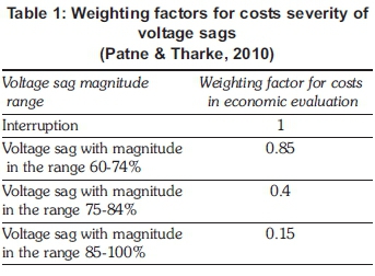
The equipment used by the customer would be affected differently by occurrence of voltage sags than would be the case by occurrence of interruptions. The latter would take all equipment out of operation. Lesser effect will occur in the case of a sag that does not culminate in an interruption. Weighting factors in Table 1 are assumed in the study to account for severity of voltage sags.

 

 

Three customer mix scenarios, as shown in Table 2, are used in the illustrative case study. The last consideration made takes into account the fact that the exposure that customers have to the interruptions is dependent on the fraction of the time that operations are carried out in a given period. The correction factors used on the study are 0, 0.238, 0.357, and 1 for residential customers, commercial customers (two days off every week, 8 hour a day operation), industrial customers (one day off per week, 10 hour a day operation) and large users (continuous process, 365 day operation), respectively.

 

 

5. Results and discussion

The results of the magnitudes of remaining voltages at on the faulted phase at the monitoring point are summarized in Figures 5 to 7. The plots presented are for faults along various lines and for different types of faults. The results for Base Case (without DG) and for case with DG are plotted side by side in each of the figures to facilitate comparison.

It is evident from the figures that for each plot for a particular fault types, the magnitudes of voltages that remain at the monitoring point are generally higher, and often significantly so, for the case with DG compared with Base Case. The positive impact of DG on improving the magnitudes of voltages is evident.

The procedure for calculating the estimated cost of critical voltage sags was introduced in Section 2 and in Table 3 illustrative results, obtained for the case of a single phase fault and the assumption of a 0.8 per unit kV sensitivity criterion, are presented.

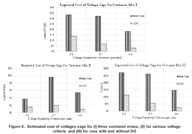
Further to the results in Table 3, the outcomes of the analysis of expected of cost critical voltage sags for various customer mixes are presented in Figure 8. For each mix, results are provided for various voltage sensitivity criterion.

It is evident that as the voltage sensitivity criterion is tightened (i.e., increased), the expected cost of critical voltage sags generally increases. The exception to this is the 0.8 per unit kV case for customer mix II, where costs are lower than for the other two criteria.

This apparent deviation can be resolved with the aid of equation (8) which shows that net expected cost of voltage sags is influenced by an interaction between the number of voltage sags, which tends to increase the costs, and the severity of voltage sags, represented by weighting factors that decreases as the severity of sags decreases.

A comparison of the expected costs for the DG Case and Base Case, for all the customer mixes evaluated, show that the costs are consistently lower for the DG Case compared with the Base Case for all voltage sensitivy criteria.

 

6. Conclusions

The results of a study into the impact of distributed generation on the expected cost of voltage sags was presented. A stochastic approach, using method of fault positions, was used to predict voltage sag performance from which expected number of critical voltage sags/annum and ultimately the expected cost/annum has been derived.

It was demonstrated that with the incorporation of DG, in relation to the case without DG, the magnitudes of voltages that remain in the system following faults are improved, with the expected number of critical voltage sags being reduced. Substantial reduction in the expected cost of voltage sags was achieved.

It was shown that, in addition to documented benefits of incorporating DG resources in power systems, the DG improved voltage sag performance, reduced the likelihood of interruptions of production, as well as reduced associated expected financial losses.

 

Acknowledgements

The authors wish to express their appreciation to the University of Johannesburg and Eskom Holdings SoC Limited for the support given to the project.

 

References

Akorede M. FF, Hizam H., Aris I., Kadir M. Z. A. and Pouresmaeil E. (2010). Economic viability of distributed energy resources relative to substation and feeder facilities expansion, in Proc. 2010 IEEE International Conference on Power and Energy (PECon2010), Nov 29 - Dec 1, 2010, Kuala Lumpur: Malaysia: 238-242.         [ Links ]

Bollen, M. H. J. (2000). Understanding power quality problems: Voltage sags and interruptions. IEEE Press Series on Power Engineering, The IEEE, lnc., New York: USA.         [ Links ]

Bollen M. H. J., Yalcinkaya G., Pellis J. and Qader M. R. (1996). A voltage sag study in a large industrial distribution system, in Proc. 31st IEEE Industry Applications Conference, San Diego: USA: 1-6.         [ Links ]

Dugan, R. C., McGranaghan, M. FF, Santoso, S. and Beaty, H. W. (1996). Electrical power systems quality, 2nd Edition. McGraw-Hill, New York: USA.         [ Links ]

Garcia-Martinez S. and Espinosa-Juárez E. (2008). Analysis of distributed generation influence on voltage sags in electrical network, in Proc. 3rd International Multi-Conference on Engineering and Technological Innovation, (IMETI 2010), June 29- July 2, 2010, Florida: USA: 1-6.         [ Links ]

Gil H. A. and Joos G. (2008). Models for quantifying the economic benefts of distributed generation. IEEE Transactions on Power Systems, 23(2): 327-1335.         [ Links ]

Hambley A. R., (2014). Electrical engineering: principles and applications, 6th Edition. Pearson Education Limited, Essex: England.         [ Links ]

Ipinnimo, O., Chowdhury S., Chowdhury S. P, and Mitra I. (2013). Review of voltage dip mitigation techniques with distributed generation in electricity networks. Electric Power System Research, 103: 28-36.         [ Links ]

Juarez E. and Hernandez A. (2006). An analytical approach for stochastic assessment of balanced and unbalanced voltage sags in large systems. IEEE Transactions on Power Delivery, 21(3): 1493-1500.         [ Links ]

Milanovic J. V. and Gupta C. P (2006). Probabilistic assessment of financial losses due to interruptions and voltage sags-part I: The methodology. IEEE Transactions on Power Delivery, 21(2): 918-924.         [ Links ]

Milanovic J. V. and Gupta C. P. (2006). Probabilistic assessment of financial losses due to interruptions and voltage sags-part II: Practical implementation. IEEE Transactions on Power Delivery, 21(2): 925-932.         [ Links ]

Moschakis M. N. and Hatziargyriou N. C. (2006). Analytical calculation and stochastic assessment of voltage sags. IEEE Transactions on Power Delivery, 21(3): 1727-1734.         [ Links ]

Nodushan M. M., Ghadimi A. A., and Salami A. (2013). Voltage sag improvement in radial distribution networks using reconfiguration simultaneous with DG placement. Indian Journal of Science and Technology, 6 (7): 4682-4689.         [ Links ]

Patne N. and Tharke K. L., (2010). Effect of transformer type on estimation of financial loss due to voltage sag-PSCAD/EMTDC study. IET Generation, Transmission, and Distribution, 4(1): 104-114.         [ Links ]

Ramos A. C. L. , Batista A. J., Alvarenga B. P, and Leborgne R. C. (2014). A first approach on the impact of distributed generation on voltage sags studies, in Proc. International Conference on Renewable Energies and Power Quality (ICREPQ'14), University of Cordoba: Spain, Paper 432: 1-6.         [ Links ]

Ramos A. C. L., Batista A. J., Leborgne R. C. and Emiliano P H. M. (2009). Distributed generation impact on voltage sags, in Proc. Brazilian Power Electronics Conference 2009 (COBEP 09), 27 September -1 October 2009, Bonito-Mato Grosso do Sul: Brazil: 446-450.         [ Links ]

Renders B, Gussemé K. D., Ryckaert W. R, Stockman K, Vandevelde L, and Bollen M. H. J (2008). Distributed generation for mitigating voltage dips in low-voltage distribution grids. IEEE Transactions on Power Delivery, 23(3): 1581-1588.         [ Links ]

Rojas H. E, Cruz A. S., and Rojas H. D. (2013). Voltage sags assessment in distribution systems using distributed generation, in Proc. SICEL VII Simposio Internacional sobre Calidal de la Energia Electrica, 27-29 Noviembre 2013, Medellin: Colombia: 1-6.         [ Links ]

Thasananutariya T. and Chatratana S. (2005). Stochastic prediction of voltage sags in an industrial estate, in Proc. IEEE Proceedings, Industrial Applications Conference, Kowloon: Hong Kong: 1489-1496.         [ Links ]

Thasananutariya T. and Chatratana S. (2005). Investigation of voltage sags due to faults in MEA's distribution system, in Proc. 18th International Conference on Electricity Distribution (CIRED 2005), Turin: Italy: 1-5.         [ Links ]

Wackerly D.D., Mendenhall W., and Scheaffer R. L. (2008). Mathematical Statistics with Applications, 7th Edition, Thompson Higher Education: Carlifornia, 2008.         [ Links ]

PSS/E (2009). Power System Simulator for Engineering: Online Documentation : Ver. 32, Siemens Energy, Inc.         [ Links ]

 

 

* Corresponding author. Email: jhcpretorius@uj.ac.za
Tel: +27 31 559 3377