A comparative study of the stochastic models and harmonically coupled stochastic models in the analysis and forecasting of solar radiation data

 

 

Edmore Ranganai^I; Mphiliseni B Nzuza^II

^IDepartment of Statistics, University of South Africa, Florida Campus, South Africa
^IISchool of Mathematics, University of Zululand, KwaDlangezwa, South Africa

 

 

---

ABSTRACT

Extra-terrestrially, there is no stochasticity in the solar irradiance, hence deterministic models are often used to model this data. At ground level, the Box-Jenkins Seasonal/Non-seasonal Autoregressive Integrated Moving Average (S/ARIMA) short memory stochastic models have been used to model such data with some degree of success. This success is attributable to its ability to capture the stochastic component of the irradiance series due to the effects of the ever-changing atmospheric conditions. However, irradiance data recorded at the earth's surface is rarely entirely stochastic but a mixture of both deterministic and stochastic components. One plausible modelling procedure is to couple sinusoidal predictors at determined harmonic (Fourier) frequencies to capture the inherent periodicities (seasonalities) due to the diurnal cycle, with SARI-MA models capturing the stochastic components. We construct such models which we term, harmonically coupled SARIMA (HCSARIMA) models and use them to empirically model the global horizontal irradiance (GHI) recorded at the earth's surface. Comparison of the two classes of models shows that HCSARIMA models generally out-compete SARI-MA models in the forecasting arena.

Keywords: irradiance, Box-Jenkins methodology, harmonic, periodogram, forecasting

---

 

 

1. Introduction

Sunshine levels, incident on a photovoltaic (PV) panel have the overriding influence on electrical output. This output is affected by the unpredictability of the prevailing whether conditions, which in turn, leads to the fluctuating nature of the solar resource. Hence, its efficient use requires reliable forecast information of its availability in various time and spatial scales depending on the application. Forecasts are critically important for use in monitoring solar systems, energy system sizing and optimization and utility applications. Utilities and independent system operators use forecasting information to manage generation and distribution. Therefore, appropriate solar data modelling and reliable forecasting of solar radiation is essential for the design, performance prediction and monitoring of solar energy conversion systems. One class of models used successfully in the literature to achieve this are the short memory Box-Jenkins Seasonal/Non-Seasonal Autoregressive Integrated Moving Average (S/ARIMA) stochastic models (Craggs et al., 1999; Zaharim et al., 2009; Voyant et al., 2013a).

In the forecasting domain, literature shows that S/ARIMA models out-competed many competing models. Pedro and Coimbra (2012) found that the improvement in 2-hours ahead forecasting using the ARIMA model with respect to the persistent model as measured by the decrease in Root Mean Squared Error (RMSE) was comparable to that of Artificial Neural Networks (ANN), i.e., 10.3% and 11.3% respectively. Reikard (2009) compared the S/ARIMA model to five other forecasting techniques in predicting high resolution data and found the SARIMA models to give the best results in four out of six test stations in the study. Actually, in the literature S/ARIMA and ANN models are considered to be the most preferred prediction methods (Alados et al., 2007; Altandombayci and Golcu, 2009; Balestrassi et al., 2009).

Extra-terrestrially, there is no stochasticity in the solar irradiance, hence, deterministic models are often used to model this data. At ground level, the success of SARIMA models is attributed to their ability to capture the stochastic component of the irra-diance series due to the effects of the ever-changing atmospheric conditions. However, such irradiance data recorded at the earth's surface is rarely entirely stochastic as weather phenomena cause varying degrees of stochasticity and deterministic components in solar irradiance. One plausible modelling procedure is to couple sinusoidal predictors at determined harmonic (Fourier) frequencies to capture the inherent periodicities (seasonalities) due to the diurnal cycle with SARIMA models capturing the stochastic components. To model this unpredictable mixture, Badescu et al. (2008) used a sinusoidal predictor to model seasonality and then represented the resulting standardized residuals by an ARMA model. However, this approach is limiting. We therefore generalize this approach by combining a sinusoidal predictor(s) to model major sea-sonalities and then fitting SARIMA models to the resulting residuals. We term this class of models Harmonically Coupled SARIMA (HCSARIMA) models. Another motivation for the proposal of HCSARIMA models is that ARMA models give unacceptable errors for distant horizon forecasting such as for more than 2 hours in the hourly case and 2 days in the daily case (Voyant et al., 2013b). In order to minimize the forecast errors for a longer horizon, i.e., 2 cycles-ahead (28 and 24 hours in the case hourly data; 168 and 132 10-minutely intervals for 10-minutely data (see Table 1)), in the SARIMA models we include seasonal parameters to model seasonality while in HCSARIMA models the major seasonalities are modelled by sinusoidal components. By modelling the seasonality in this way, distant horizon forecasts of up to 24 hours or more essential for power dispatching plans, optimization of grid-connected PV plants and coordination control of energy storage devices (Wang et al., 2012) will be valid as seasonal models are able to capture the entire seasonal swing.

We undertake a comparative study of these two classes of models viz., SARIMA versus HCSARIMA in modelling and forecasting the horizontal solar irradiance (GHI) (comprising of both direct normal irradiance (DNI) and diffuse horizontal irradiance (DHI)) data series recorded at the University of KwaZulu-Natal (UKZN) Howard College (HC) campus (Durban, South Africa) Faculty of Engineering's recently established (February, 2010) radiometric broadband ground station. This station is located at 29.9° South, 30.98° East with elevation, 151.3m. Measurements recorded were obtained from the Greater Durban Radiometric Network (GRADRAD) database (www.gradrad.ukzn.ac.za). A shadow band type Precision Spectral Pyranometer (Model PSP) is used to obtain the three irradiances. The DHI obtained by blocking the direct solar beam must be corrected for additional sky band blockage; hence the DNI obtained by subtraction from GHI is less accurate than that obtained from Pyrheliometers. Therefore, we study the more accurate GHI.

Although most of the studies in the literature used a calendar year's historical data series (Zalwilska and Brooks, 2011) to learn repeatable patterns that may be inherent in the series, in some instances it is also useful to use a shorter historical data series to learn strongly fluctuating patterns that may be inherent in a shorter period such as a season, month or less (Craggs et al., 1999; Yona et al., 2013). We follow the later approach and make use of the February (summer) and July (winter) 2011 data series. The data series are in two time scales, viz., hourly and 10-minutely which we adjudged to provide a fair compromise between the now-casting solar irradiance problem on very short time intervals (15 seconds to 30 minutes) and one day ahead forecasts crucial for controlling a PV plant operation (Paulescu et al., 2013).

In the next section, we give a brief overview of SARIMA models. In Section 3 we elaborate on the periodogram as well as its use in searching for periodicities in data series leading to the building of the HCSARIMA model. Model selection based on in-sample diagnostics and forecasting accuracy are given in Section 4, data series modelling is carried out in Section 5, model comparisons are carried in Section 6 and conclusions are given in the last section.

 

2. SARIMA Models

The generalized form of a multiplicative SARIMA model can be specified as

(Cryer and Chan, 2008), where

are the seasonal AR, non-seasonal AR, seasonal MA and non-seasonal MA factors, respectively, the constant δ coincides with the mean of the series and S is the seasonality. The operator, L is the backward shift operator such that L^kX_t - X_t__k, d and D are the non-seasonal and seasonal order differences, respectively, taking positive integer values. For instance, (1 - L)^d X_t = Δ^dX_t - X_t - X_t-1 and (1 - L^S')^DX_t = Δ^D/_SX_t = X_t - X_t-sfor d = D = 1. The powers PS, p, QS and q denote the seasonal AR, non-seasonal AR, seasonal MA and non-seasonal MA orders, respectively. It is assumed that Z_t is white noise, i.e., Ζ_t~N (0,σ²_Z). This model in (2.1) is usually abbreviated as SARIMA (p, d, q) X (P, D, Q)_S. Note that the seasonal and non-seasonal AR and MA factors in (2.1) may be additive.

To build SARIMA models via the Box-Jenkins methodology (Box and Jenkins, 1976), time domain techniques are made use of. On the other hand, to build HCSARIMA models spectral methods (periodogram analysis) are used to determine the inherent periodicities in the data series.

 

3. The periodogram

Frequency Domain techniques are used to search for periodicities in data. The standard tool to carry out such an analysis is called the spectrum, which is a Fourier transform of the autocorrelation function (ACF). In practice, the sample estimator of the spectrum, the periodogram first introduced by Schuster (1898), is used to determine periodicities in data. An efficient way to compute the periodogram is to make use of the Fast Fourier transform (FFT) (Chatfield, 2003). For a realization of a time series, , the periodogram is defined as:

where are harmonic frequencies, is the FFT and [.] denotes the integer part. Using the well-known result from the analysis of variance (ANOVA), the total sum of squares (SST) of the series can be partitioned into sum of the error terms (SSE) plus sum of squares due to a periodic component (I(ω_p)). viz.,

Dividing (3.2) by η throughout clearly, a large contribution of the sum of squares due to the periodic component to SST implies a large contribution to the variance of the series by I(ω_ρ) (Chatfield, 2003: 127). If this is the case, then much of the variability in the data series is attributable to the periodic component.

3.1 Searching for periodicities and construction of the HCSARIMA model

Suppose that a time series is dominated by a periodic sinusoidal component with a known wavelength. Then the natural model is:

where ω_ρis the frequency of the sinusoidal variation, R is the amplitude of the variation, ϕ is the phase and {Z_t} as in (2.1). Equivalently, (3.3) can be expressed as:

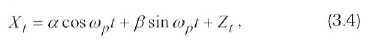
where α = Rsinϕ and β = Rcosϕwith µ_t = 0. In practice, a series may contain multiplicities of periodicities and the generalized form of (3.4) becomes

Note that ω_khas to be a harmonic frequency since ordinary least squares and ML (under normality) estimators at different general frequencies ω_K and ω_J are not independent because the sine-cosine and complex exponential systems are complete and orthogonal only over Fourier frequencies.

For the model (3.5), if in a periodogram analysis, a particular intensity Ι(ω_g) is the largest one, we can test the hypothesis whether the parameters a and β are indeed zero, at this frequency i.e.

by making use of The Fisher's Kappa statistic Fuller (1976).

To detect general departures from white noise, Bartlett's Kolmogorov-Smirnov statistic can be used. Also, the usual F-test can be used to test the significance of any periodogram ordinate of interest e.g. the 2^nd largest say I(ω_h) (Wei, 2006:292). Now, the seasonality at significant periodogram ordinates I((ω_g) is modelled by equations (3.4) or (3.5). In practice {Z_t} is rarely white noise such that it is described by a SARIMA model. The non-stationary residuals are denoted by {W,}. Thus, combining (3.4) or (3.5) with a trend component, and (2.1) gives a HCSARIMA model, viz.,

If there are multiplicities of seasonalities in the data series (3.6) becomes

where μ_tis the trend function which is dropped if nonsignificant.

 

4. Model selection criteria

Model selection criteria are two-fold, i.e., we make use of in-sample diagnostics as well model prediction accuracy measures.

4.1 In-sample diagnostics

The selection of the best SARIMA model was carried out using the principle of parsimony (select the model with the least number of parameters), high R-square value and two Information Criteria, viz., Akaike's information criterion (AIC) and the Schwarz's Bayesian criterion (SBC) (Akaike, 1983; Schwarz, 1978) also known as the Bayesian information criterion (BIC). The lower the values of these statistics the better the model is. The SBC is preferred over AIC since the AIC criterion overestimates the order of auto-regression (Wei, 2006).

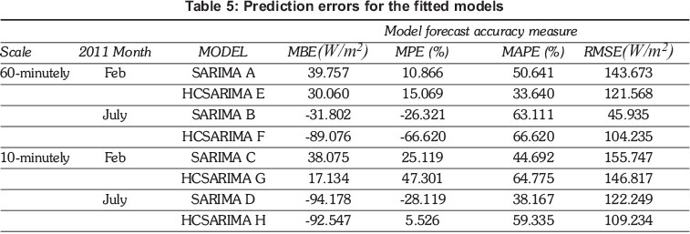
4.2 Prediction accuracy

We make use of four common measures, viz., Mean Bias Error (MBE) in W/m², Mean Percentage Error (MPE), Mean Absolute Percentage Error (MAPE) and Root Mean Squared Error (RMSE) in W/m², in assessing the model out-of-sample two 2 days (cycles)-ahead forecast errors. The smaller the values of these measures the better the forecasts. The formulations of these forecasting measures are:

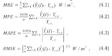
where Y_t+l and Ŷ_t(l) are the actual and forecasted / -steps ahead forecasted values, respectively.

 

5. Data modelling

All the data analysis is done using a statistical analysis system (SAS). The readings are taken instantaneously at 6 seconds intervals and then averaged minutely. We further average the minutely data in 60-minutely and 10-minutely. The details of the data series are presented in Table 1, along with their daily cycle lengths.

The February 60-minutely daily data spans from 0500 hours to 1800 hours and that for July spans from 0600 hours to 1700 hours, while the February 10-minutely daily data spans from 0500 hours to 1850 hours and that for July spans from 0630 hours to 1720 hours. Most of the missing values generally occur before around 0635 hours and after around 1725 hours for the July month. This explains the difference in the percentage of missing values between the hourly and 10-minutely July data series.

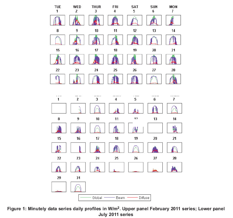
The February series from the 1^st to the 13^th and the July data series from the 3^rd to the 9^th were used for model building. The next 2 days data series was used for validation in each case. We adjudge these days to have the best data quality by making use of the following minutely data series profiles for each day of the February and July months given in Figure 1. These profiles can be obtained from http://gradrad.ukzn.ac.za .

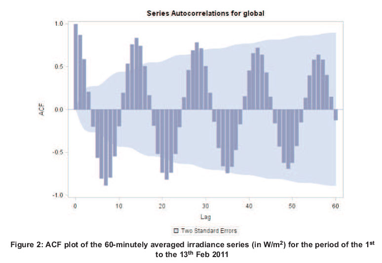
We confirm the periodicities evident by means of time domain techniques such as time ACFs (Figure 2) as well as search for hidden ones using periodogram analysis in the next subsection.

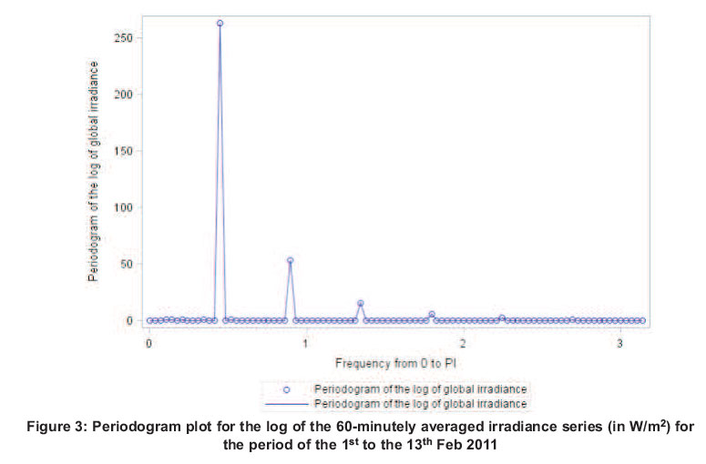
5.1 Periodogram analysis

For brevity we only give results for the February 60-minutely series. In Figure 3, the periodogram is plotted against the harmonics, ω_ρ. Table 2 shows the Fisher's Kappa test and BKS test results. Lastly, the F-test results for the same data series are given in Table 3.

 

 

 

 

The largest intensity is at period 14, the second largest is at period 7 and the third largest is at period 4.667 corresponding to harmonics ω₁₄ = 2π/14, ω₇ = 2π/7 ω₄.₆₆₆₇ = 2π/4.667, respectively. Fisher's Kappa results in Table 2 show the presence of a strong periodic component since the test statistic, 66.875, is greater than the critical value, 8.882 at the 1% level of significance while the BKS statistic has a p-value< 0.05 indicating that generally the series is not white noise, i.e., the presence of at least one periodic component. The strongest periodic component is further confirmed by the F-test (p-values< 0.05) in Table 5.3, which also shows both the second largest and the third largest ordinates to be significant.

The harmonics used in HCSARIMA models G to H in subsection 5.2 were obtained in a similar fashion.

5.2 SARIMA and HCSARIMA Modelling

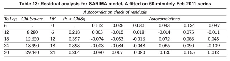
Both SARIMA and HCSARIMA models with significant (p-values< 0.05) parameters were fitted on all four data series (see Appendices A and B, respectively) via maximum likelihood (ML) estimation. To check the adequacy of these models, tables of residual analysis based the Box-Ljung statistics (p-val-ues< 0.05), histograms (bell-shaped) of residuals, Q-Q plots (approximately straight line), and the Anderson-Darling normality test (p-values < 0.05). Satisfying all criteria in parenthesis constitute adequacy. For brevity, only results for Model A are given in Appendix C.

SARIMA modelling

Parameter estimates for SARIMA models are given in Tables 4 to 7 in Appendix A. These are:

• Model A, 60-mmutel\j averaged February 2011 series:

• Model B, 60-minutelv averaged Ju/y 2011 series:

• Model C, 10-minutely averaged February 2011 series:

• Model D, on 10-minutely averaged July 2011 series:

HCSARIMA modelling

Parameter estimates for HCSARIMA models are given in Tables 8 to 11 in Appendix B. These are:

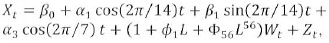
• Model E, 60-minutely averaged February 2011 series:

• Model F, 60-minutely averaged July 2011 series:

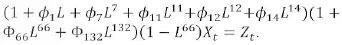
• Model G, the 10-minutely averaged February 2011 series;

Table 9 shows parameter estimates for the HCSARIMA model, G.

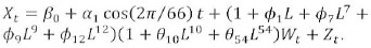
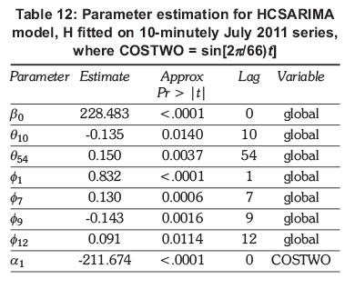
• Model H, the 10-minutely averaged July 2011 series;

 

6. Models comparison

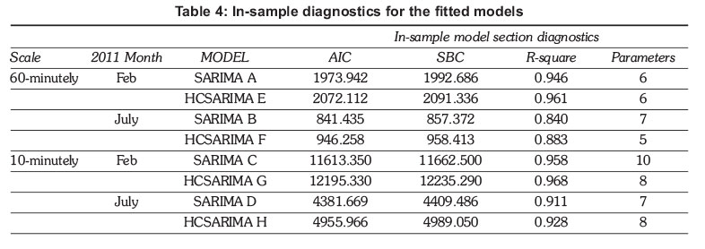
In-sample model selection diagnostics

In-sample diagnostics used here are given in Table 4 viz., AIC, SBC (BIC), R-square and parsimony. The principle of parsimony selects the model with the least number of parameters.

SARIMA Model A is superior to HCSARIMA Model E in terms of criteria AIC and BIC but inferior with respect to R-square. Furthermore, the two models are equally parsimonious.

SARIMA Model B is superior to HCSARIMA Model F in terms of the two criteria, AIC and BIC but inferior with respect to the two measures, R-square and parsimony. SARIMA Model C and HCSARIMA Model G follow a similar pattern exhibited by SARIMA Model B and HCSARIMA Model F with respect to all measures, respectively. SARIMA Model D fares better than HCSARIMA Model H with respect to all diagnostics except R-square.

Prediction

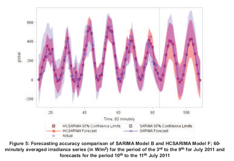
Prediction accuracy diagnostics made use of here to compare the SARIMA models and HCSARIMA models are given in Table 5 viz., MBE, MPE, MAPE and RMSE. Also, the SARIMA and HCSARIMA models are compared graphically both with respect to point estimation and the 95% confidence intervals (CIs).

SARIMA Model A is out-performed by HCSARIMA E with respect to all the prediction accuracy measures except MPE, while SARIMA Model B performs better than HCSARIMA Model F in all the given prediction accuracy measures.

For both HCSARIMA Models G and H perform better than SARIMA Models C and D with respect to the MBE and RMSE and otherwise with respect to MPE and MAPE, respectively.

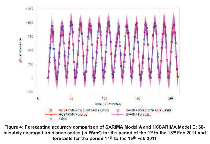
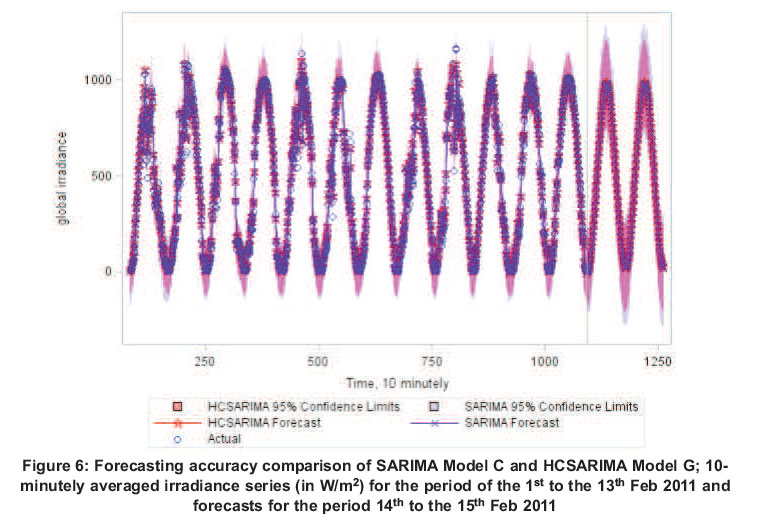
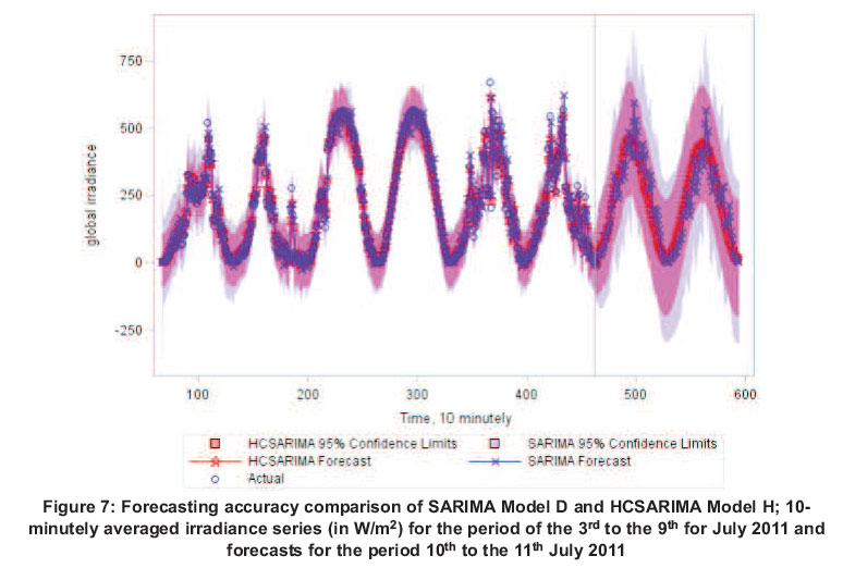
Graphically, the pair-wise forecasting accuracy comparisons of SARIMA models and HCSARIMA models are shown in Figures 4 to 7.

Note that the night times have been removed in order to get rid of the zero values.

The point forecasts of SARIMA Model A and HCSARIMA Model E in Figure 4 seem indistinguishable. However, the 95% CIs of SARIMA Model A are consistently wider than those of HCSARIMA Model E, hence the later model has a competitive. The picture is somewhat different for the 60-minutely series for July 2011, with respect to interval estimation as shown in Figure 5.

 

Table 5

 

In these series, the 95% Cls for SARIMA Model B are wider those of HCSARIMA Model F in approximately a third of the estimation data series. Thereafter, both upper and lower confidents limits (CLs) tend to be alternating in size. However, in the hold out sample the upper CLs of SARIMA Model B, are wider than those for HCSARIMA Model F and vice-versa in the case of lower CLs.

The forecasting comparisons between SARIMA and HCSARIMA models for the 10-minutely series are given in Figures 6 and 7. The two figures exhibit a pattern similar to that in Figure 5, i.e., the point forecasts of SARIMA m\Models (C and D) and HCSARIMA Models (G and H) seem indistinguishable, while the 95% CLs for SARIMA models are generally wider than those of HCSARIMA models. Therefore, the HCSARIMA models have a competitive edge to SARIMA models.

Discussion

There is no clear 'winner' between the two classes of models, viz., SARIMA and HCSARIMA models, with respect to in-sample diagnostics. Empirically, it was observed that addition of a deterministic (sinusoidal) predictor would inflate the AIC and SBC diagnostics. As a consequence, these two measures were larger for HCSARIMA models compared to SARIMA models, giving SARIMA models a competitive edge in this regard. However, the opposite was true for the in-sample measures R-square and parsimony, where the HCSARIMA models performed better. To keep the values of AIC and SBC marginally larger we had to reduce the number of deterministic predictors, i.e., allowing some periodicities to be described by SARIMA model parameters in the HCSARIMA models. Thus, it was only at the largest intensity (periodogram ordinate) that a sinusoidal predictor was used except for HCSARIMA Model E where a second sinusoidal predictor was added to model the seasonality at the second largest intensity. The addition of a sinusoidal predictor gives HCSARIMA models superiority with respect to R-square values and more or less better with respect to parsimony as HCSARIMA models have a single case of being marginally less parsimonious (HCSARIMA H).

In the prediction scenario, HCSARIMA models are found to be generally superior than SARIMA models. It is only in one data series (60-minutely July 2011) where SARIMA Model B out-performs HCSARIMA Model F in all prediction measures. Furthermore, it was in this data series where in terms of the 95% CI estimation there was no clear better class of models. Otherwise in the other three data series the HCSARIMA models were found to be better than SARIMA models in the 95% CI estimation. However, we have reservations on this outcome of SARIMA model B versus HCSARIMA Model F due to the fact that the least amount of data series was available as well as the largest proportion of missing values inherent in this case.

 

7. Conclusions

While short memory SARIMA models are useful on their own, combining them with sinusoidal deterministic predictors to form HCSARIMA models generally has some competitive advantages in the prediction arena. However, the inclusion of sinusoidal predictors results in relatively larger AIC and SBC values. Using a smaller number of sinusoidal predictors gives a reasonable balance in the trade-off between the inflation of AIC and BIC values, and the improvement in forecasting. Alternatively, another proposal around this is to use SARIMA models for data generation and then use HCSARI-MA models for forecasting. However, if the purpose of the models is only forecasting then there might be no need to restrict the number of sinusoidal predictors. In this scenario, all the harmonics found to be corresponding to significant periodogram ordinates using frequency domain techniques can be used to model the multiplicities of periodicities present.

 

Acknowledgements

Special thanks go to Michael Brooks of the UKZN School of Engineering for providing data, information and suggestions.

 

References

Akaike, H. (1983). Information Measures and Model Selection, Bulletin of the International Statistical Institute, 50, 277-290.         [ Links ]

Alados I., Gomera M.A., Foyo-Moreno I., and Alados-Arboledas L. (2007). Neural network for the estimation of UV erythemal irradiance using solar broadband irradiance. Int. J. Climatol., 27(13), 1791-9.         [ Links ]

Altandombayci O, and Golcu M. (2009). Daily means ambient temperature prediction using artificial neural network method: a case study of Turkey. Renew. Energy, 34(4), 1158-61.         [ Links ]

Balestrassi P, Popova E., Paiva A., and Marangonlima J. (2009). Design of experiments on neural network's training for nonlinear time series forecasting. Neurocomputing, 72(4-6), 1160-78.         [ Links ]

Box, G. E., and Cox, D. R. (1964). An analysis of transformations. J. Roy. Statist. Soc. Ser. B 26:211-252.         [ Links ]

Box, G. E. P and Jenkins, G. M. 1976. Time Series Analysis: Forecasting and Control, Revised ed. USA, Holden-Day Inc.         [ Links ]

Chatfield C. (2003). The Analysis of Time Series: An Introduction, 6^th Edition, Chapman & Hall/CRC Press, London.         [ Links ]

Craggs, C., Conway, E. and Pearsall N. M. (1999). Stochastic modelling of solar irradiance on horizontal and vertical planes at a northerly location. Renewable Energy 18, 445-463.         [ Links ]

Cryer D.J. and Chan K, (2008). Time Series Analysis with Applications in R, 2^nd Ed. Spring Street, New York Inc.         [ Links ]

Davis H. T. (1941). The Analysis of Economic Time Series. Indiana: The Principia Press, Inc. Bloomington.         [ Links ]

Fuller W. A. (1976). Introduction to Statistical Time Series. New York: John Wiley & Sons.         [ Links ]

GRADRAD: The Greater Durban Radiometric Network. http://gradrad.ukzn.ac.za.         [ Links ]

KZN Green Growth. http://www.kzngreengrowth.com.         [ Links ]

Paulescu, M., Paulescu, E., Gravila P. and Badescu V. (2013). Weather Modelling and Forecasting of PV Systems Operation. Springer Verlag, London        [ Links ]

Schwarz, G. (1978). Estimating the Dimension of a Model, The Annals of Statistics, 6, 461-464.         [ Links ]

Pedro H. T. C. and Coimbra C. FM. (2012). Assessment of forecasting techniques for solar power production with no exogenous inputs. Solar Energy, 86, 2017-2028.         [ Links ]

Reikard G. (2009). Predicting solar radiation at high resolutions: A comparison of time series forecasts, Solar Energy, 83, 342-349.         [ Links ]

Schuster, A. (1898). On the investigation of hidden periodicities with application to a supposed 26 day period of meteorological phenomena, Terrestrial Magnetism and Atmospheric Electricity, 3 13-41.         [ Links ]

Voyant C., Muselli M., Paoli C. and Nivet M. (2013a.) Hybrid methodology for hourly global radiation forecasting in Mediterranean area. Renewable Energy, 53, Complete, 1-11.         [ Links ]

Voyant C., Randimbivololona P., Nivet M. L., Paolic C. and Musellic M. (2013b). Twenty four hours ahead global irradiation forecasting using multi-layer perceptron. Meteorol. Appl., (2013), DOI: 10.1002/met.1387.         [ Links ]

Wei W. W. S. (2006). Time Series Analysis. Univariate and Multivariate Methods. 2^nd Ed. Addison Wesley.         [ Links ]

Yona A., Senjyu T., Funabashi T., Mandal P and Kim C-H. (2013). Decision Technique of Solar Radiation Prediction Applying Recurrent Neural Network for Short-Term Ahead Power Output of Photovoltaic System. Smart Grid and Renewable Energy, 2013, 4, 32-38.         [ Links ]

Zaharim A., Razali A. M., Gim, T. P. and Sopian, K. (2009). Time Series Analysis of Solar Radiation Data in the Tropics. European Journal of Scientific Research. .25, 672-678.         [ Links ]

Wang F., Mi Z., Su S. and Zhao H. (2012). Short-Term Solar Irradiance Forecasting Model Based on. Artificial Neural Network Using Statistical Feature Parameters. Energies, 5, 1355-1370.         [ Links ]

Zawilska E. and Brooks M.J. An Assessment of the Solar Resource for Durban, South. Africa. Renewable Energy, 36:12, 3433-3438.         [ Links ]

 

 

Received 31 October 2013
Revised 11 December 2014

 

 

Appendix A: ML estimation for SARIMA models

 

 

 

 

 

 

 

 

Appendix B: ML Estimation for HCSARIMA Models

 

 

 

 

 

 

 

 

Appendix C: Checking adequacy for Model A

 

Table 13 - Click to enlarge

 

 

Figure 8 - Click to enlarge