Mapping wind power density for Zimbabwe: a suitable Weibull-parameter calculation method

 

 

Tawanda Hove^I; Luxmore Madiye^II; Downmore Musademba^III

^IDepartment of Mechanical Engineering, Faculty of Engineering, University of Zimbabwe, Harare, Zimbabwe
^IIDepartment of Mechanical Engineering, Faculty of Engineering, University of Zimbabwe
^IIIDepartment of Fuels and Energy, School of Engineering Sciences and Technology, Chinhoyi University of Technology, Zimbabwe

 

 

---

ABSTRACT

The two-parameter Weibull probability distribution function is versatile for modelling wind speed frequency distribution and for estimating the energy delivery potential of wind energy systems if its shape and scale parameters, k and c, are correctly determined from wind records. In this study, different methods for determining Weibull k and c from wind speed measurements are reviewed and applied at four sample meteorological stations in Zimbabwe. The appropriateness of each method in modelling the wind data is appraised by its accuracy in predicting the power density using relative deviation and normalised root mean square error. From the methods considered, the graphical method proved to imitate the wind data most closely followed by the standard deviation method. The Rayleigh distribution (k=2 is also generated and compared with the wind speed data. The Weibull parameters were calculated by the graphical method for fourteen stations at which hourly wind speed data was available. These values were then used, with the assistance of appropriate boundary layer models, in the mapping of a wind power density map at 50m hub height for Zimbabwe.
Keywords: Weibull distribution parameters, graphical method, power density.

Keywords: Weibull distribution parameters, graphical method, power density.

---

 

 

1. Introduction

The energy performance analysis and economic appraisal of wind energy conversion systems require knowledge on the probabilistic distribution of wind speed, apart from just knowledge on the mean wind speed. Knowing the probability density distribution, one can assess the economic viability of installing a wind energy conversion system at a particular location (Celik et al, 2010; Antonio et al., 2007) Various theoretical mathematical representations of probability distribution functions have been published in the literature (Ramirez and Carta, 2005; Mathew et al., 2002; Seguro and Lambert, 2000; Garcia et al., 1998; Littella et al., 1979), such as the Rayleigh, lognormal and two-parameter unimodal Weibull probability distribution functions.

Although the bimodal Weibull pdf, Jaramillo and Borja (2004) might produce a better fit on the wind speed data, especially for some locations in Zimbabwe which experience frequent null wind speeds, its use is regarded as an unnecessary addition to complexity where only the power density of the wind is required. This is because the first mode of the frequency distribution appears at null or very low wind speeds which are not important in producing useful power considering that the cut-in speed of wind turbines is typically between 7 and 10 mph (about 3 to 4.4 m/s) (Glynn, 2000). This study will therefore focus on the two-parameter unimodal Weibull probability density function for imitating wind speed frequency distribution at the sites in question. The parameters k (the shape factor) and c (the scale factor) of the two-parameter Weibull distribution will be determined by some of the various methods found in the literature.

Mathew (2006) gives a concise description of five methods that could be used to determine the values of the two-parameter Weibull distribution. The methods are; the graphical, the standard deviation, the moment, the maximum likelihood and the energy pattern factor (EPF) methods. Harrison, Cradden and Chick (2007) note that the Rayleigh distribution, which is a simplification of the Weibull distribution in which k=2, and is defined solely by mean wind speed, is often applied where specific data for k is not available. Indeed it is relied upon in many studies where time series data is not available and the Weibull parameters cannot be determined. In this paper, the Rayleigh distribution is also considered alongside the other aforementioned distributions to assess its suitability in imitating the actual wind speed data.

The criterion for assessing the suitability for each method in modelling wind speed data is its ability to estimate closely the power density at the site. The theoretical maximum power density achievable by any wind turbine - Betz Limit (van Kuik, 2007; Gorban et al; 2004; Hughes and George, 2002) - is used as a common yardstick for the comparison.

 

2. The Weibull distribution

The frequency distribution of wind speed at a given site can be modelled by the two-parameter Weibull probability density function (pdf). The Weibull pdf, p_W [s/m], can be written:

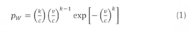
In (1), v is the wind speed (in units of speed; m/s or knots). k, the shape factor, is dimensionless, and specifies how sharp a peak the Weibull curve has. The parameter, c [m/s], the scale factor, is the weighted average speed; more useful for power calculations than the actual mean speed (Gorban et al, 2004). The parameters k and c vary from site to site and have to be determined for each site to fit wind speed frequency distribution for the site.

In terms of the mean wind speed, , and k. the pdf can be written (Ramirez and Carta, 2005) as:

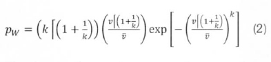
The function.[x, is the gamma function of x. Comparing (1) and (2), it can be observed that the mean speed, is given by:

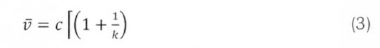
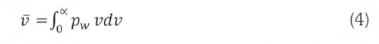
If k and c are known, hence the functional relationship of p_wand v known, the mean wind speed can be obtained from numerical integration of the expression:

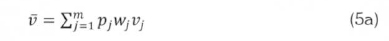
For the measured wind data grouped in m classes of class width, w_j[m/s], (j=1 to m), and class probability density, p_j [s/m], the mean, , and standard deviation, σ, for measured data are given respectively by:

and

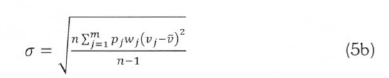
In (5) V_j is the class centre speed of the j^th class. For class frequency, fj, the class frequency density for a sample population of n wind speed records is obtained as:

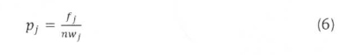
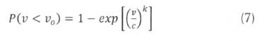
The cumulative pdf can be obtained by integrating (1) from 0 to any value of v; say v_o.

The power density [W/m²] of a wind turbine is given by:

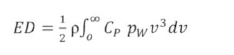
In (8). p is the air density [kg/m³], and is considered constant at a given turbine height. The power coefficient, Cp, is an empirically determined function of wind speed v for a given turbine. The maximum power coefficient, independent of turbine design, is given by the Beta limit (Mathew, 2006; van Kuik, 2007; Gorban et al. 2004):

Therefore, the maximum power density is given by:

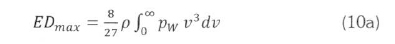
for the Weibull distribution, and

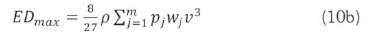
for grouped data.

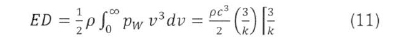
The integral in (10a) can be solved analytically (Mathew, 2006), but can conveniently be solved numerically with the advent of various spreadsheet programs. The analytical integral for wind power density, ED, is given by:

The maximum power density computed by (10a) for the Weibull functions generated from different methods, can be compared with that of (10b), for the measured wind data, in appraising a given method's accuracy in imitating the measured wind data. Another way for comparing the accuracy of the methods is by comparing the normalised root mean square error, NRMSE. The NRMSE is given in general by:

 

3. Data available for study

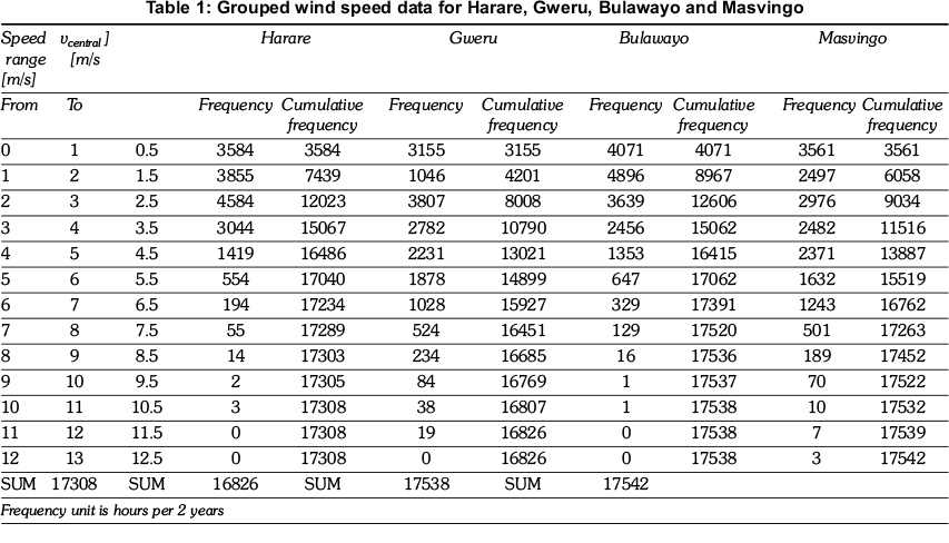
The finest time-step resolution of wind speed measurements available in Zimbabwe is the hour. Hourly wind speed data is available at only fourteen stations over all of Zimbabwe. Such data was obtained for two years (1991 - 1992), from the Meteorological Services Department (MSD) of Zimbabwe. The measurements are done by cup anemometers placed at a height of 10 m above ground. For each station, the data was subsequently grouped into speed-spectra frequency bins of 1 m/s range to prepare for later analysis. The grouped data for four major stations is shown in Table I for validation of the methods described in Section 4.

The models used for determining the diurnal variation of energy output for the two generating components of the hybrid system; PV array and diesel generator, are outlined in this section.

 

4. Methods for determining Weibull parameters from wind data

Mathew (2006) describes five different methods for determining the values of the Weibull k and c from measured wind data. These methods, namely; the graphical; the standard deviation; the moment; the maximum likelihood and the energy pattern factor methods, are reviewed in the following sections and are going to be used to determine k and c values from the data in Table I. In addition, the commonly used Weibull simplification- the Rayleigh distribution- is tested for its goodness-of-fit on the measured data.

4.1 Graphical method

The graphical method for determining k and c is based on the fact that the Weibull cumulative distribution function of (7) can be transformed into a log-linear form, and the technique of linear regression exploited. The cumulative pdf is manipulated by taking natural logarithms twice on both sides to make it a linear equation. The resulting equation is:

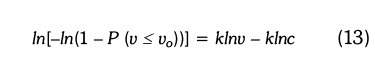
Equation (13) is linear in ln[-ln(1 - P (v < v_o))], the dependent variable (Y), and lnv, the independent variable (X) in Y = a + bX, in which a = -klnc and b = k are regression constants.

Hourly meteorological records of wind can now be grouped in speed -spectra frequency bins or classes, and the values of ln[-ln(1 - P (v < v_o))] and lnv_ocalculated for each class.

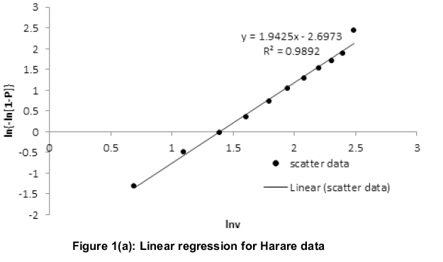
The symbol v_ois the upper limit speed value of the class, and P, for each class, is the number of speed records with speed lower than v_o, divided by the total number of records in the sample (-the relative cumulative frequency). Log-linear regression fits are shown on Figures 1(a) and 1(b), for Harare and Gweru respectively.

The gradient of the regression line in Figures 1(a) and 1(b) equals the value of k, and the intercept equals -klnc, from which c can be inferred. The graphs show a very strong correlation of the variables with the coefficient of determination, R², about 0.99 in each case.

At P = 1, the natural logarithm of 1-P does not exist. In this case, 1-P is replaced by a a very small number, essentially zero, but not equal to zero, such that the logarithm of 1-P is computable.

4.2 The standard deviation method

The method used for the UK Wind Energy Program (WindPower and UK Wind Speed Database, 2012), called by (Mathew. 2006) the standard deviation method, relates to the ratio of the standard deviation, a, to the mean speed, v, (-the coefficient of variation), with the parameter k as follows:

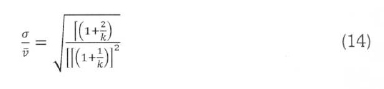
Equation (14) is not explicit in terms of k and can only be solved by numerical methods. However, (Justus et al.. 1978) provide a simpler approximation for k.

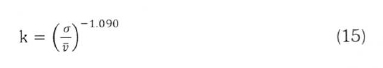
The mean, and standard deviation, o, are obtained from the wind data using (5). Having determined k from the wind statistics, c can be evaluated by transforming (3) into:

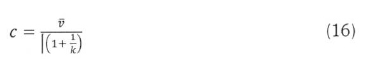
To evaluate c in (15), we have to evaluate the gamma function of 1 + 1/k, which is rather complex. However, some common spread sheet programs such as Microsoft Excel include the natural logarithm of gamma in their function library. In Excel, the natural logarithm of gamma is denoted by the function name "GAMMALN". Gamma is then the exponential of GAMMALN.

Alternatively, Justus et al. (1978) give the following approximation expression:

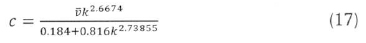
With both k and c evaluated as above, the Weibull function of (1) can be generated.

4.3 Moment method

Another method for estimating k and c is the First and Second Order Moment Method, where the nth moment M_n of the Weibull distribution is given by Mathew (2006):

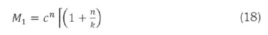
If M₁ and M₂ are the first and second moments, c can be solved as:

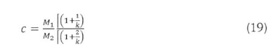
Similarly, k can be solved from (18) and (19) by eliminating c, with:

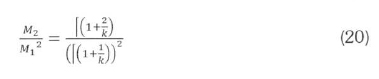
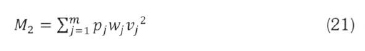
M₁ and M₂ are calculated from the given wind speed data from the statistical fact that the moment is the expected value of a positive integral power of a random variable. Thus, M₁ is equal to the mean. . and is evaluated by (5a). The second moment M₂ is computed for grouped data as:

A numerical solution for k is required using (20). and then c is evaluated from (19).

4.4 Maximum likelihood method

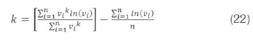
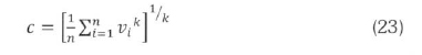
In the maximum likelihood method, the Weibull parameters, k and c, are given by Cohen (1965) and Ananstasios et al. (2002):

and

The summations in (22) and (23) are replaced for grouped data as follows:

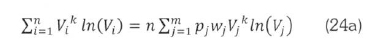
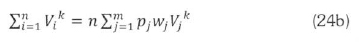
and

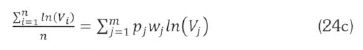
Now, in (22), k is not expressed explicitly, and has to be solved numerically. First, a value k (any number between 0 and 2 will do), and evaluate the summations on the right hand side of (22) or their simplified versions in (24). The value of k is varied until its value is such that (22) is satisfied. After getting a satisfactory k. the parameter c is preferably evaluated from (3) to retain consistency with the Weibull formula.

4.5 Energy pattern factor method

The Energy Pattern Factor (EPF) is the ratio of the total power available in the wind and the power corresponding to the cube of the mean wind speed (Mathew. 2006). That is:

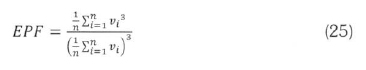
In the grouped data format, the energy pattern factor can be written as:

Once EPF is calculated from (25). the parameter k is approximated as:

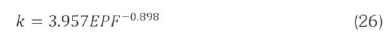
The parameter c can be calculated from Equation (3) once k is obtained.

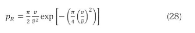
4.6 Rayleigh distribution

In some cases where time series wind is not available but only long-term statistics like the mean wind speed are known, the aforementioned methods cannot be applied. It is common under these circumstances to assume that the Rayleigh distribution is a suitable proxy of the real distribution. The Rayleigh distribution is a simplified form of the Weibull distribution in which k=2. With this assumption, rearranging (3) and simplifying gives:

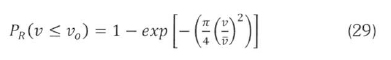
Therefore, for the Rayleigh distribution, (1) becomes:

and the corresponding cumulative distribution is:

The validity of the Rayleigh simplification in modelling wind speed data is tested, alongside the other previously discussed methods, and the results are presented in the following section.

 

5. Results

The probability density functions generated by methods described in sections 4.1 to 4.6 are compared with the measured probability density function in Figures 2(a) to 2(d) for four sample stations, Harare, Gweru, Bulawayo and Masvingo, respectively. The comparisons for cumulative probability functions are shown in Figures. 3(a) and 3(b) for Bulawayo and Masvingo, respectively.

The calculated probability density functions are uni-modal, but for some sites, as is depicted for Gweru and Masvingo (a continuous curve used to give better impression), the measured distributions are bimodal. However, the first modes of these bimodal distributions occur at low wind speed (in the 0 to 1 m/s range). Using a uni-modal distribution to represent them is considered not to seriously affect power calculations.

The theoretical distributions in Figures 2(a)-2(d) and Figures 3(a) and 3(b) (cumulative distributions are shown only for Bulawayo and Masvingo) appear to imitate the measured distribution with varying capability in doing so. However, only a subjective appraisal can be made on the relative fitness of each method to the measured data from these pictorial presentations. A quantitative comparison is required.

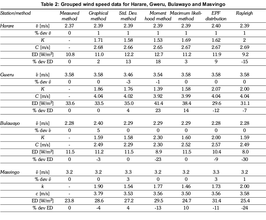
To quantitatively appraise of the various methods, Table 2 is constructed. It shows the measured mean wind speed calculated according to (5a) in comparison to the mean wind speed of the theoretical distributions of methods in sections 4.1 to 4.6, computed by (4). The table shows the percent deviation of the mean speeds from the measured. Importantly, the table also makes similar presentations for the Betz-limit power density. The corresponding values of k and c are also shown on the table.

With the aid of Table 2 it can be shown that, if the power density is considered the figure of merit, the graphical method (maximum power density deviation of 4%) is the most reliable of all methods considered, followed closely by the standard deviation method (maximum deviation of 13%). All the six methods predict the actual mean speed fairly accurately (within 5%). This is expected since, except for the graphical method all the other distributions are formulated based on the mean wind speed.

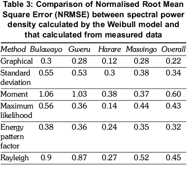
The accuracy of the methods in predicting spectral power density can also be compared by calculating the normalised root mean square error (NRMSE) for each method. The power density for each wind speed spectrum calculated by the Weibull model is compared with that calculated from measured data and a NRMSE is obtained for each sample station and for all stations combined (overall). The NRMSE values for each method are listed in Table 3. The graphical method gives the least NRMSE of all the methods for all stations.

 

 

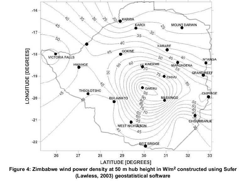
The wind power density at 50 m hub height is shown in Figure 4. To obtain the wind power density map of Figure 4, the values of k and c at the fourteen stations having hourly wind data were calculated using the graphical method. Equation (11) was then used to compute the power density at the stations, first at the measurement height of 10 m hub height, then at 50 m by applying the three-seventh-power law. The values of power density were then mapped using the ordinary kriging interpolation option of the software Surfer Version 12 (Scientific Software Group, 2013).

The wind power density for Zimbabwe is seen to be highest in the central region - the Midlands province. The power density at 50 m hub height varies between about 10 W/m² to 120 W/m². These power density levels are rather low for economical large-scale power production, lying in Class 1 of the US NREL wind power density classification (Wind Power Class, 2014). Some specially selected sites, however, may be suitable for applications such as water pumping or even power generation using special wind turbines which have low cut-in speeds.

 

6. Summary and conclusion

The study uses five different methods for calculating the parameters of the two-parameter Weibull distribution from measured wind speed data at fourteen locations in Zimbabwe. The Rayleigh distribution, which is a commonly used proxy to wind speed distributions, is also generated and compared with the measured data. The graphical method, for correlating the measured wind speed probability distribution with the theoretical Weibull distribution, estimated power density to within 4% of the actual in all the four illustrative cases considered. This method was then used to determine the Weibull parameters at the rest of the fourteen stations with hourly wind speed data. This enabled the mapping of wind power density over Zimbabwe. The wind power density for Zimbabwe is generally low for power generation purposes. Some considerable potential exists though in the Midlands province for applications such as water pumping that can do with low wind speed. The approach used in this study can be replicated in other countries in the region in creating their respective wind power density maps.

 

Acknowledgement

The authors are grateful for the financial support given by the University of Zimbabwe Research Board. The Research Grant provided enabled, among other things, the purchase of wind speed data from the Meteorological Service Department of Zimbabwe.

 

References

Ananstasios, B., Dimitrios, C., and Thodoris, D. K. (2002). A nomogram method for estimating the energy produced by wind turbine generators, Solar Energy, Vol. 72, No. 3, pp. 251-259.         [ Links ]

Antonio, J., Carta, A., and Ramirez, P (2007). Use of finite mixture distribution models in the analysis of wind energy in the Canarian Archipelago, Energy Conversion and Management, vol. 48, no. 1, pp. 281-291.         [ Links ]

Celik A. N., Makkawi A., and Muneer T. (2010). Critical evaluation of wind speed frequency distribution functions. Journal of Renewable and Sustainable Energy 2:1, 013102.         [ Links ]

Cohen, A. C. (1965). Maximum likelihood estimation in the Weibull distribution based on complete and censored data, Technometrics, Vol. 7, No. 4, pp. 579-588.         [ Links ]

Garcia, A., J. Torres, J. L., Prieto, E., and de Franciscob, A. (1998). Fitting wind speed distributions: a case study, Solar Energy, Vol. 62 No. 2, pp.139-144.         [ Links ]

Glynn, M. (2000). Zimbabwean wind spins at Redhill, Home Power, No. 76, pp. 52-54.         [ Links ]

Gorban, A. N., Gorlov, A.M., and Silantyev, V. M. (2004). Limits of turbine efficiency for free fluid flow, Energy Resources Technology, vol. 123, no. 4, 311-317, 2001. Renewable Energy, Vol. 29, No. 10, pp. 1613-1630.         [ Links ]

Harrison, G. P, L. C. Cradden, L. C., and Chick, J. P (2007). Preliminary assessment of climate change impacts on the UK onshore wind resource, Invited paper for Special Issue of Energy Sources and Global Climate Change and Sustainable Energy Development.         [ Links ]

Hughes, L., and George, A., (2002), The Weibull distribution. Available on: www.nsweep.electricalcomputerengineering.dal.ca/tools/Weibull.html, Accessed on: 20 February 24, 2013.         [ Links ]

Jaramillo, O.A. and M. A. Borja, M.A. (2004). Wind speed analysis in La Ventosa, Mexico: a bimodal probability distribution case, Renewable Energy, vol. 29, no. 10, pp. 1613-1630.         [ Links ]

Justus, C. G., Hargraves, W. R., Mikhail, A., and Graber, D. (1978). Methods of estimating wind speed frequency distribution, J. Applied Meteorology, Vol. 17, pp. 350-353.         [ Links ]

Littella, R. C., Mc Clavea, J. T., and Offena, W. W. (1979). Goodness-of-fit for the two-parameter Weibull distribution, Communications in Statistics -Simulation and Computation, Vol. 8, No. 3, pp. 257-259.         [ Links ]

Mathew, S. (2006). In: Wind energy fundamentals, resource analysis and economics, Berlin, SpringerVerlag, Chapter 3.         [ Links ]

Mathew, S., Pandey, K. P. and Kumar, A. (2002). Analysis of, wind regimes for energy estimation, Renewable Energy, Vol. 25, No. 3, pp. 381-399.         [ Links ]

Ramirez, P., and Carta, A. (2005). Influence of the data sampling interval in the estimation of the parameters of the Weibull probability density functions: a case study, Energy Conversion and Management, Vol. 46, Nos. 15-16, pp. 2419-2438.         [ Links ]

Scientific Software Group, Surfer 12 for Windows. Available at: http://www.ssg-surfer.com. Accessed on 24 January 2013.         [ Links ]

Seguro, J. V., and Lambert, T. W. (2000). Modern estimation of the parameters of the Weibull wind speed distribution for energy analysis, Journal of Wind Energy and Industrial Aerodynamics, vol. 85, no. 1, pp. 75-84.         [ Links ]

The WindPower and UK Wind Speed Database programs (online). Available on: http://www.wind-power-program.com/wind_statistics.htm. Accessed 12 December 2012.         [ Links ]

van Kuik, G. A. M. (2007). The Lanchester-Betz-Joukowsky limit, Wind Energy, Vol. 10, pp. 289-291.         [ Links ]

Wind Power Class - Wind Energy Resource Atlas of the United States. Available at: http://rredc.nrel.gov/wind/pubs/atlas/tables/1-1T.html. Accessed 30 September, 2014.         [ Links ]

 

 

Received 11 December 2013
Revised 11 October 2014