RESEARCH ARTICLE

 

Modelling influence of temperature on daily peak electricity demand in South Africa

 

 

Delson Chikobvu^I; Caston Sigauke^II

^IDepartment of Mathematical Statistics and Actuarial Science, University of the Free State, South Africa
^IISchool of Statistics and Actuarial Science, University of the Witwatersrand, South Africa

 

 

---

ABSTRACT

The paper discusses the modelling of the influence of temperature on average daily electricity demand in South Africa using a piecewise linear regression model and the generalized extreme value theory approach for the period - 2000 to 2010. Empirical results show that electricity demand in South Africa is highly sensitive to cold temperatures. Extreme low average daily temperatures of the order of 8.20C are very rare in South Africa. They only occur about 8 times in a year and result in huge increases in electricity demand.

Keywords: Extreme value theory, piecewise linear regression, regression splines, temperature.

---

 

 

1. Introduction

Drivers of electricity demand are generally divided into economic factors, calendar effects, weather variables and lagged demand variables. Inclusion of these factors in electricity demand models improves the predictive power of the models and also enables system operators and load forecasters to have a better understanding of the factors that have a greater impact on electricity demand. Weather variables such as temperature, solar radiation, humidity, wind speed and rainfall are often used as explanatory variables in regression based load forecasting models. Most authors, however, use temperature as the main driver (Munoz et al., 2010).

The influence of temperature on daily electricity load forecasting has been studied extensively in the energy sector using classical time series, regression based methods including artificial neural networks (Miragedis et al., 2006; Hekkenberg et al., 2009; Psiloglou et al., 2009; Munoz et al., 2010; Pilli Sihvola et al., 2010; among others). The paper discusses the modelling of the effect of average daily temperature on daily electricity demand in South Africa using a piecewise linear regression modelling framework and the generalized extreme value theory approach. A generalized extreme value distribution (GEVD) is fitted to the temperature data below the reference temperature. Extreme value theory (EVT) is a powerful and fairly robust framework for modelling the tail behaviour of a distribution (Gencay and Selcuk, 2004). Extreme value theory has been applied in various fields such as flood frequency analysis, environmental sciences, modelling extreme temperatures, finance and insurance including material and life sciences. The family of extreme value distributions is called the generalized extreme value distribution. GEVD consists of the Gumbel, Frechet and Weibull class distributions which are also known as the type I, II and III extreme value distributions respectively.

The rest of the paper is organized as follows. The models are discussed in Section 2. In Section 3 we briefly describe the data used. Empirical results are presented in Section 4 while Section 5 concludes.

 

2. The models

Our modelling approach is in two stages. A piecewise linear regression model is used to explore the effect of temperature on daily electricity demand. In stage two, we fit a generalized extreme value distribution to the temperature values below the reference temperature. The fitted distribution is then used to estimate extreme low temperatures and calculating the corresponding marginal increases of electricity demand.

2.1 Piecewise linear regression model

The piecewise linear regression model used for modelling the influence of temperature on electricity demand is given in equation (1).

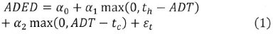
where ADED (Average Daily Electricity Demand), ADT (Average Daily Temperature), th and tc are temperatures which separate summer and winter sensitive periods (hot and cold temperatures) from the weather neutral period respectively. The parameters to be estimated are α₀, α₁ and α₂ and ε_t is the error term with ε_t~N(0,σt²). A Multivariate Adaptive Regression Splines (MARS) algorithm developed by Friedman (1991) is used to estimate the two reference temperatures tc and th which are 18°C and 20°C respectively and discussed in Chikobvu and Sigauke (2012).

2.2 Generalized extreme value distribution

The GEVD consists of the Gumbel, Frechet and Weibull class of distributions. The unified GEVD for modelling maxima is given by

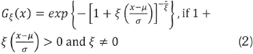
where µ and σ are the location and scale parameters respectively. The shape parameter ξ also known as the extreme value index (EVI) determines the rate of tail decay. If ξ > 0, G_ξ(x) belongs to the heavy-tailed Frechet class of distributions (Beirlant et al., 2004). For ξ < 0 we have the short-tailed Weibull class and is bounded above by (Beirlant et al, 2004). If ξ = 0, G_ξ(x) belongs to the light-tailed Gumbel class of distributions (Beirlant et al, 2004).

In order to model minima we use the duality between the distributions for maxima and minima. If M_n = min{x₁, x₂, ..., x_n} where x_i, i = 1,2, ..., n represents temperature, then M_n = max{-x₁, -x₂, ..., - x_n}. Extreme maxima theory and methods are then used to model extreme minima. The Maximum Likelihood (ML) method is used to estimate the parameters ξ, μ and σ. The survival distribution of the GEVD given in equation (2) is given by:

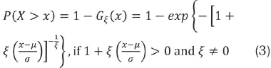
If we let p = P(X > x) and rearranging equation (3) to make x the subject we get the quantile function:

Now as p → 0 and ξ < 0 we get . The quantile function for the unified GEVD given in equation (4) is then used to estimate high quantiles and predicting the probability of exceedance levels.

 

3. Data

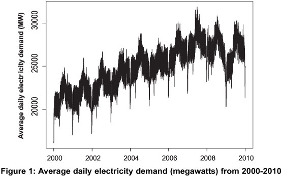
National daily electricity data for the industrial, commercial and domestic sectors of South Africa is used in this study. The data is from Eskom, South Africa's power utility company. Figure 1 shows that ADED data exhibits strong seasonality and has a positive upward trend.

 

 

Aggregated ADT from 32 meteorological stations of South Africa representing all provinces (regions) of the whole country is used in the analysis.¹

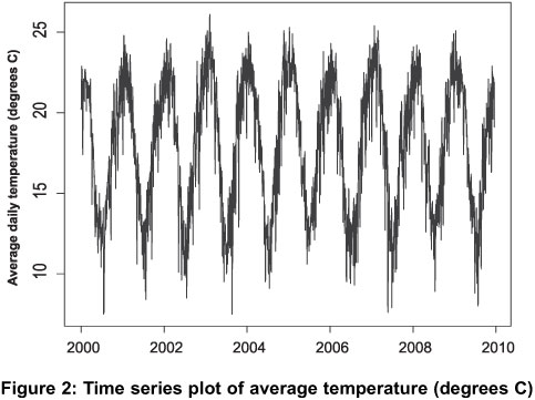
Figure 2 shows that ADT has strong seasonality and is stationary. The minimum ADT and maximum ADT over the sampling period (2000-2010) are 7.5⁰C and 26.1⁰C respectively.

 

 

4. Empirical results and discussion

4.1 Piecewise linear regression model output

The model identifies the winter sensitive, weather neutral and summer sensitive periods. The model is not used for forecasting electricity demand but rather to explain the influence of temperature on electricity demand.

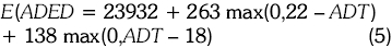
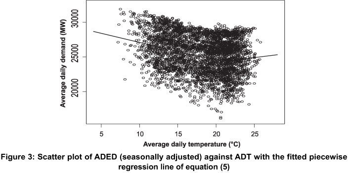
The graphical plot of ADED against ADT is shown in Figure 3. The three demand-temperature equations are given in equations 6-8. If average daily temperature is less than or equal to 18⁰C equation (5) reduces to

That is, if the temperature decreases by 1⁰C (e.g. from 18⁰C to 17⁰C) electricity demand will increase marginally by 263 MW. A fall in ADT of 1⁰C (say, from 16⁰C to 15⁰C) would result in an increase of about 1.03% in electricity consumption.

If average daily temperature is greater than or equal to 22⁰C equation (5) reduces to

If temperature increases by 1⁰C (e.g. from 22⁰C to 23⁰C) electricity demand will increase marginally by 138 MW. For a rise in average daily temperature of 1⁰C (say, from 25⁰C to 26⁰C) would result in an increase of about 0.55% in electricity consumption.

For the average daily temperature between 18⁰C and 22⁰C we use the full model given in equation (5), i.e.

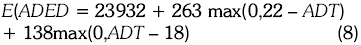
If temperature decreases by 1⁰C (e.g. from 22⁰C to 21⁰C) electricity demand will increase marginally by 125 MW. A decrease of ADT from 20⁰C to 19⁰C would result in an increase of about 0.51% in electricity consumption.

This analysis shows that electricity demand in South Africa is highly sensitive to cold temperature (see Figure 3). There is a non-linear relationship between temperature and electricity demand as shown in Figure 3. This non-linear relationship is modelled in literature using heating degree days (HDD) and cooling degree days (CDD). Modelling of this relationship between temperature and electricity demand is discussed in literature (Mirasgedis, 2006; Franco and Sanstad, 2008; Psilogu et al., 2009; Munoz et al., 2010; Pilli-Sihvola et al., 2010; among others). HDD and CDD are calculated using the following functions:

where ADT is the average daily temperature at time and is the reference temperature.

In this paper a piecewise linear regression model is used with two reference temperature values which are estimated using the MARS algorithm (Friedman, 1991).

Figure 3 shows the plot of the model in equation (5). The piecewise linear regression plot separates the non-linear response of electricity demand to temperature into three regions: cold for temperatures lower than 18⁰C, neutral for temperatures between 18⁰C and 22⁰C, and hot for temperatures above 22⁰C.

There are other several methods of filtering data (i.e. removing both the trend and the calendar effects) which are discussed in literature (see Moral-Carcedo and Vic'ens-Otero, 2005; Munoz et al., 2010; among others).

4.2 Modelling the minimum daily temperature (tail quantile estimation)

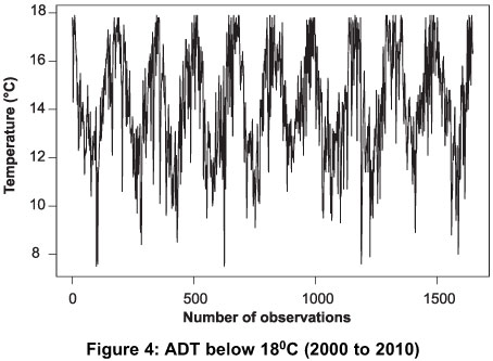
In section 4.1 it was noted that demand of electricity is more sensitive to cold temperatures (less than 18⁰C) than to hot temperatures (more than 22⁰C). Modelling of extreme minimum temperatures is therefore important to load forecasters and system operators for planning, load flow analysis and scheduling of electricity. In this section, we estimate the extreme tail quantiles of ADT below 18⁰C using the GEVD. The data is seasonally adjusted. There are 1649 observations below 18⁰C. Figure 4 shows data for temperature below 18⁰C.

 

 

4.3 Tail quantile estimation

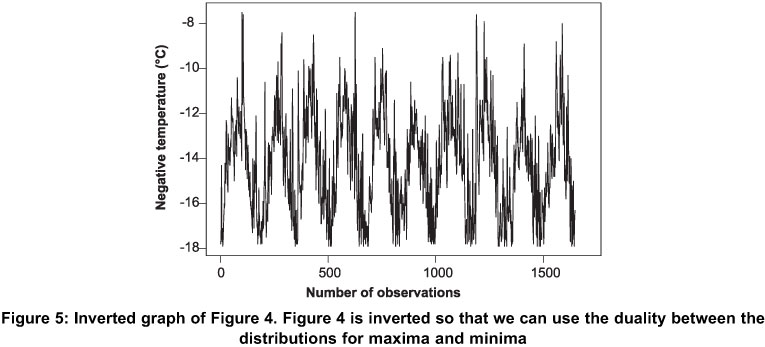
We use the principle of duality between the distributions of minima and maxima as discussed in Section 2.2. Figure 5 shows the graph of -x_i, i = 1, ...,n where x_i represents temperature below 18⁰C. The R statistical package Ismev (Heffernan and Stephenson, 2013) is used to obtain the ML estimates. The estimates are given as (the standard errors are given in parentheses):

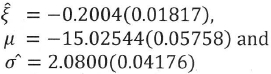
The standard errors of the ML estimates of the parameters, are small. This shows that uncertainty about the parameters is small. These results show that the data can be modelled using a Weibull class of distributions, (since ) and the right endpoint is finite and is given by:

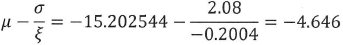
This implies that for any degree decrease below 4.6⁰C there won't be any further increase in electricity demand.

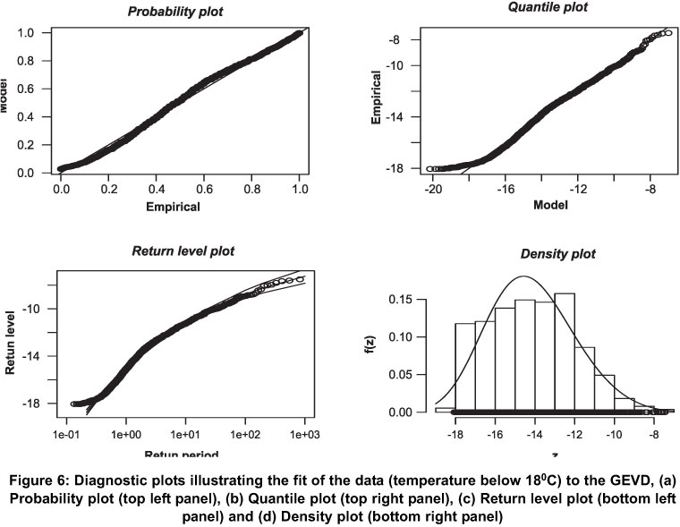
The quantile-quantile (QQ) and probability-probability (PP) plots given in Figure 6 show that a Weibull distribution is a good fit to the data. The return level estimates are inside the 95% confidence interval. This is an indication that the fitted distribution is capable of accurately predicting future return levels. We then use equation (4) to estimate the future return levels for different return periods. The return level is the quantile of the GEVD (Weibull distribution). For example, the 95^th quantile is obtained as follows:

The number of observations that are smaller than the estimated tail quantile (x_0.05 = 10.369) are then counted and found to be 78. For the observed number of exceedances, we get 0.05 x 1649 = 82.45 ≈ 82 where 1649 is the number of temperature values below 18⁰C. The increase in electricity demand for a drop of temperature from 18⁰C to x_0.05 = 10.4°C is given by (18 - 10.4) x 263 = 1998.8MW, where 263 is the marginal increase in demand for a decrease of 1⁰C below 18⁰C as discussed in Section 4.1. It should be noted that this increase in ADED for temperature decreases below 18⁰C is bounded above. As temperature decreases below 18⁰C, the increases in ADED reaches a certain maximum after which any further decrease in temperature will not have any effect on ADED. That is as temperature decreases people will switch on heating systems up to a point when all the heating systems are all switched on and no additional energy is consumed.

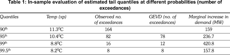
Table 1 presents a summary of the estimated tail quantiles at different tail probabilities. The tail quantiles (temperature) are given in column 2. The observed number of observations (temperature) that are smaller than the estimated tail quantiles are shown in column 3 while column 4 shows the corresponding number estimated using GEVD. In equation (5) it is given that for a degree decrease in temperature below 18⁰C there will be a marginal increase in demand of 263 MW. For each of the estimated quantiles in column 2, column 5 shows the marginal increases from one quantile to the next, e.g. if temperature drops from 11.3⁰C to 10.4⁰C there will be an increase in demand of 263(11.3 - 10.4) = 236.7MW. Similarly, for a decrease from 10.4⁰C to 8.8⁰C the marginal increase will be 263(10.4 -8.8) = 420.8MW. Extreme low average daily temperatures of the order of 8.2⁰C are very rare in South Africa. This only occurs about 8 times in a year.

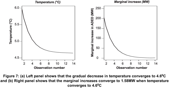
Table 2 given in the Appendix summarizes the temperature values at high quantiles and the corresponding marginal increases while Figure 7 shows that the marginal increases converge to 1.58 MW when temperature converges to 4.6⁰C.

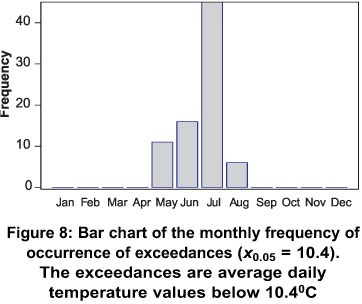
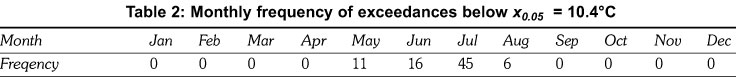
A summary of the monthly frequency of occurrence of temperature values below 12.4⁰C (i.e. above the 95^th quantile -x_0.05 = 10.369 is given in Table 2. Over the sampling period, i.e. years 2000 to 2010 the month of July has the highest number of days with temperature values below 10.4⁰C. This is an indication that the month of July is the coldest month in South Africa and the winter period is from May to August of each year.

The bar chart of the monthly frequency of occurrence of exceedances is given in Figure 8.

 

 

5. Conclusion

An analysis of the intensity and frequency of occurrence of extreme low temperatures is important for load forecasters in the electricity sector. In this paper, the modelling of the influence of temperature on average daily electricity demand in South Africa using a piecewise linear regression model and the extreme value theory modelling framework is discussed. The developed piecewise linear regression model is not meant for forecasting but to model the effect of temperature on electricity demand. The study establishes temperature as an important variable in explaining electricity demand. Empirical evidence from this study shows that for temperature values below 18⁰C demand for electricity in South Africa increases significantly while for temperature values above 22⁰C demand increases slightly. This analysis is important for decision makers in Eskom, South Africa's power utility company. Extreme low temperatures can be modelled by the Weibull class of distributions. Extreme low temperatures of the order of 6⁰C are very rare in South Africa, but can cause huge increases in electricity demand. An investigation of expected- cooler or warmer than typical years is important and helps in guiding planning to decision makers in the electricity sector.

Areas for future research would include a comparative analysis of the generalized extreme value distribution with a generalized Pareto distribution and a generalized single Pareto distribution in modelling extreme low temperatures in South Africa. These areas will be studied elsewhere.

 

Note

1. Average daily temperature for the whole country is usually built into the modelling as weighted average temperatures from different meteorological stations of a country. The weightings should reflect consumption of electricity of each region (province). Population figures are often used for estimating the weights. In this research, the weightings were not done since only aggregated average daily temperature was available.

 

Acknowledgments

The authors are grateful to Eskom for providing the data and to the numerous people who assisted in making comments on this paper.

 

References

Chikobvu, D. and Sigauke, C., (2012). A frequentist and Bayesian regression analysis to daily peak electricity load forecasting in South Africa. African Journal of Business Management, 6(40): 10524-10533.         [ Links ]

ClimateTemp.info. (Accessed on 10 June 2012) www.climatetemp.info/south-africa/.         [ Links ]

Franco, G. and Sanstad, A.H. (2008). Climate change and electricity demand in California. Climatic Change, 87 (Suppl 1): S139-S151.         [ Links ]

Heffernan, J.E. and Stephenson, A.G. (2013). Ismev: R package version 1.39.         [ Links ]

Hekkenberg, M., Benders, R.M.J., Moll, H.C. and Schoot, A.J.M. (2009). Indications for a changing Electricity demand pattern: The temperature dependence of electricity demand in the Netherlands, Energy Policy, 37: 1542-1551.         [ Links ]

Gencay, R. and Selcuk, F (2004). Extreme value theory and value-at-risk: relative performance in emerging markets. International Journal of Forecasting, 20: 287-303.         [ Links ]

Hyndman, R.J., Fan, S. (2010). Density forecasting for long-term peak electricity demand. IEEE Transactions on Power Systems, 25(2): 1142-1153.         [ Links ]

Mirasgedis, S., Sarafidis, Y., Georgopoulou, E., Lalas, D.P, Mschovitis, M., Karagiannis, F and Papakonstantinou, D. (2006). Models for mid-term electricity demand forecasting incorporating weather influences. Energy, 31: 208-227.         [ Links ]

Moral-Carcedoa, J. and Vic'ens-Otero, J. (2005). Modelling the non-linear response of Spanish electricity demand to temperature variations. Energy Economics, 27, 477-494.         [ Links ]

Munoz, A., Sanchez-Ubeda, E.F, Cruz, A. and Marin, J. (2010). Short-term forecasting in power systems: a guided tour. Energy Systems, 2: 129-160.         [ Links ]

Pilli-Sihvola, K., Aatola, P, Ollikainen, M. and Tuomenvirta, H. (2010). Climate change and electricity consumption Witnessing increasing or decreasing use and costs, Energy Policy, 38(5), pp. 2409-2419.         [ Links ]

Psiloglou, B.E., Giannakopoulos, C., Majithia, S. and Petrakis, M., (2009). Factors affecting electricity demand in Athens, Greece and London, UK: A comparative assessment. Energy, 34: 1855-1863.         [ Links ]

SouthAfrica.info. (Accessed on 10 June 2012) southafrica.info/travel/advice/climate.htm.

www.ral.ucar.edu/~ericg/softextreme.php.

 

 

Received 1 October 2012
Revised 21 November 2013

 

 

Appendix

 

Tabela 2 - Click to enlarge