


Services on Demand
Article
 English (pdf)
 Article in xml format
 Article references
Indicators

Related links
-
 Cited by Google
 -
 Similars in Google
Share

 Permalink
Journal of Energy in Southern Africa
On-line version ISSN 2413-3051
Print version ISSN 1021-447X
J. energy South. Afr. vol.24 n.1 Cape Town Jan. 2013
The significance of relevance trees in the identification of artificial neural networks input vectors
G Manuel; JHC Pretorius
University of Johannesburg
ABSTRACT
In the 1980s a renewed interest in artificial neural networks (ANN) has led to a wide range of applications which included demand forecasting. ANN demand forecasting algorithms were found to be preferable over parametric or also referred to as statistical based techniques. For an ANN demand forecasting algorithm, the demand may be stochastic or deterministic, linear or nonlinear. Comparative studies conducted on the two broad streams of demand forecasting methodologies, namely artificial intelligence methods and statistical methods has revealed that AI methods tend to hide the complexities of correlation analysis. In parametric methods, correlation is found by means of sometimes difficult and rigorous mathematics. Most statistical methods extract and correlate various demand elements which are usually broadly classed into weather and non-weather variables.
Several models account for noise and random factors and suggest optimization techniques specific to certain model parameters. However, for an ANN algorithm, the identification of input and output vectors is critical. Predicting the future demand is conducted by observing previous demand values and how underlying factors influence the overall demand. Trend analyses are conducted on these influential variables and a medium and long term forecast model is derived. In order to perform an accurate forecast, the changes in the demand have to be defined in terms of how these input vectors correlate to the final demand. The elements of the input vectors have to be identifiable and quantifiable. This paper proposes a method known as relevance trees to identify critical elements of the input vector. The case study is of a rapid railway operator, namely the Gautrain.
Keywords: artificial neural networks, input vectors, demand forecast, relevance trees, Gautrain rapid railway system, notified network demand
1. Introduction and research motivation
For many high end energy consumers, special agreements are formulated between the electrical consumer and electrical supplier. One such high energy consumer was the operating company of South Africa's new commuter railway system, namely the Gautrain. The electric commuter railway system is supplied by means of a Main Propulsion Substation (MPS) for which the point of supply is 88kV. The MPS supplied the commuter boggies with power through the pantograph by means of a distribution network. This is a 25kV pantograph which was constructed in line with international standards (BS EN 50163 and IEC 60850). Several studies reiterate the importance of a demand forecast. Here, the importance of a demand forecast is for the supply agreement. Supply authorities reserve a stipulated demand for the industrial consumer and high demand consumer. This is referred to as the Notified Network Demand (NND).
The supply agreement usually requires a forecast of two entities; namely the monthly energy consumption and NND. The NND is defined as the maximum demand at any given time. This may only be altered over a twelve month rolling period. Both underestimation and overestimation of the NND leads to a loss of revenue. Overestimation of the demand at any given time means that excess capacity is reserved that is not being utilized. In the case of under estimation, revenue loss may be the result of penalties being awarded by the supplier to the consumer for exceeding the stipulated demand. This emphasizes the importance of a demand forecast for this particular consumer and several other industrial or high electrical energy demand consumers. An Artificial Neural Network (ANN) was selected as the method for which to formulate a demand forecasting algorithm. ANN forecasting methods have become the focal point of several studies and academic papers in recent years. ANN is one of several artificial intelligent driven methods inspired either by human intuition or the human biological system. The advantage of most AI derived algorithms is the ability to process and model nonlinear processes with the added benefit of generality. Statistical models define the demand by means of identifying underlying rhythms or cycles and the factors that affect these cycles (mostly in terms of weather and non-weather factors). Correlation of these factors leads to a forecast model. Selected parametric models account for noise and stochastic or stationary process within the demand. Some may be capable of modelling only the peak demand (NND) and may not necessarily model the demand curve (energy demand). The area under the demand curve defines the energy consumption and holds the most interest from a consumer point of view.
ANN hides the complexities of defining each rhythm and how these influential factors are correlated onto the final magnitude of the demand. The demand and its factors are simply correlated by means of a learning process. ANN models may consist of several layers. The first layer is the input layer and the last layer the output layer. The output layer identifies the information that is needed (demand at time t). In determining the final outcome, the input vectors become vital. But how are these input vectors determined? For the output vectors, the requirements were derived from the supply agreement. These were the demand curve (energy demand) and peak demand (identifies the NND).
The ANN paradigm can be defined in terms of a correlation type of algorithm defining a linear and nonlinear demand in terms of the influences on the input vectors. Several papers identify the knowledge base approach as a vital prerequisite for the demand forecast algorithm. This is because by having adequate knowledge of the demand, suitable input parameters may be identified. The input vectors must be relevant to the factors that define the demand or influence it. If these factors are not fully accounted for then an accurate forecast may not be determinable. Apart from the identification of input parameters, quantification and acquisition of the magnitude of these parameters are of paramount importance. Certain parameters may be easily identified and quantified of which the most common variable is being weather variables. Many forecast models account for the weather as being a significant component. A good example of this is the following regression model defined by three components:
![]()
LPh,d: The potential demand component
LWh,d: The weather demand component
LIh,d: The irregular demand component
h: Identifier for the time of day
d:Identifier for the type of day (special days and weekdays)
Regression models generally define the demand in terms of weather and non-weather components. However the influential factors that affect the demand component can be further subdivided into several more components. The advantage of ANN based forecast models are that the correlation of each input vector, be it weather or non-weather variables is not explicitly formulated. Instead a series of learning patterns cause the model to correlate the variables with parameters that derive the final demand. The rail system was developed through a sequence of simulation models. These models provided unrealistic results since the model input parameters were not fully understood or quantified.
The objective of this paper is to present a method of identifying demand parameters to be used as input vectors for the ANN forecast model. Even though many experts advise about the benefits of first understanding the nature of the demand prior to the development of a demand forecast model, this is not always possible. The operator of the newly developed commuter rail system was not the same company or contractors that were responsible for the construction and commissioning of the railway link. A series of test runs were undertaken before the system was opened for normal commuter operations. However, these were under no commuter demand conditions. Transit systems require more tractive effort as compensatory measures due to an increase in the train weight in order to overcome upward and downward forces. Another significant factor not easily simulated. Henceforth, this paper briefly discusses ANN and relevance trees and how input elements of the input vector were identified for the ANN demand forecast algorithm.
2. Artificial neural networks
The study of artificial neural networks (ANN) was inspired by the human biological system. The human nervous system consists of a finite amount of neurons that make up the human biological system (illustrated in Figure 1). In the biological neural network, dendrites receive signals from other neurons in the form of electrical pulses. These signals then flow along the axon ending up at the synapse. These pulses are either inhibited or exited depending on whether the summation of all signals received by the synapse are above a threshold level. In terms of what is described here thus far, the artificial neural network is very much comparable. Figure 1 illustrates a single artificial neuron. Here, synapses are now replaced with inputs and dendrites with outputs. The neuron is excited when the summated value of the inputs are greater than the threshold value, else the neuron is inhibited. Not all inputs are considered equal. Each input has an associated weight which increases the value of the input. In this manner, the significance of particular demand element that accounts for the most changes in the demand is accounted for at that particular time. For a single neuron to fire or excite, equation 1 holds true:

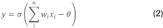
Where:
y: define the output
x: define the inputs
w: define the weights
σ: activation function
θ: bias term
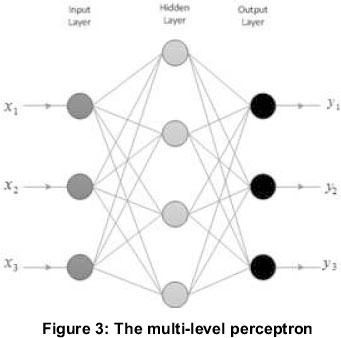
An artificial neural network can be regarded as a parallel and distributed processor comprising out of several layers of neurons. The first layer is referred to as the input layer and the last layer the output layer. Between the input and output layer, up to several layers may exist. These are referred to as hidden layers (Illustrated in Figure 3). The topology of a multi-layer perceptron consisting of various layers is illustrated. Several papers discuss general guidelines in the selection of how many hidden layers are required as a function of the complexity of the process. The statistical subject of correlation and regression analysis is concerned with analysing the relationship between two quantitative variables. In statistical studies, correlation refers to how strongly two variables relate to one another. A high, correlation defines that two or more variables have a strong relationship with each other while a weak, or low, correlation means that the variables are hardly related. For a neural network, a series of patterns are presented to the inputs and through the process of learning a solution is converged to produce an output.
ANN learns the dependencies or correlation that quantifiable factors have on the final demand. Depending on the type of learning method employed, the networks learn how to converge onto an accurate output based upon the amendment of weight values. Hence, the choice of inputs become critical since demand variations (outputs) are defined as a dependence of the inputs in order to accurately correlate or converge onto a solution. Learning algorithms are generally subcategorized into two classes, namely supervised and unsupervised learning. In supervised learning, a set of training data (or patterns) are presented to a neural network with random weights. Training can be executed after each pattern is presented (one by one approach) or when all patterns or vectors have been presented (batch approach). The weights are then adjusted to bring about a minimum error whereby the most optimum solution is found (Least Error Squares: LES by means of gradient descent). Most critical is the direction of the error (positive or negative) in order to know in which direction the weights should be adjusted. The process whereby one pattern is learnt and the weights are adapted is referred to as iteration. The accuracy of the model is now tested with the ability of the model to accurately determine the future demand based upon the correlation of inputs to demand or outputs vectors for which it has learnt during the training phase. ANN are best known for their ability to generalize and data (magnitudes of inputs vectors) not modelled or presented before may be forecasted with a degree of accuracy based upon the correlation of previously understood data. The concept of ANN learning is an important concept and only one method is discussed here, namely the common back propagation algorithm. The difference between the net or actual output and desired output is used to formulate an error term that is used to adjust weights. This is given by:
![]()
Where:
Net: actual net output
d: desired output as given by the training data
The pattern is presented and the results are fed forward, the error is propagated backwards for error correction. The net output is calculated as the product of weights and inputs. These examples are only one common type of neural network learning topology. Several papers discuss the compilation, applications and benefits of ANN, specifically in the context of demand forecasting. Optimization techniques are also extensively presented by a general survey of available literature studies.
These forecast algorithms in many cases lack adaptability between one electrical consumer to the next. This is due to the fact that significant factors that define the demand may not be appropriately modelled. Although many papers emphasize the importance of a knowledgeable selection of inputs that define the demand, few papers present methods of achieving this. For this particular study, a classical type of knowledge based approach proved to be problematic. Relevance trees were used as these methods employ analytical techniques to analyse the demand and determine the factors that may affect the final magnitude of the demand at any given time.

3. Relevance trees and applied methodology
A relevance tree is used to map broad subject matter into several streams in order to present a graphic outline of the system. First, the highest level to be modelled is identified. This may seem like a seamless task; however, the consumer demand may be derived by means of two instances, namely a source approach or a demand base approach. In terms of a demand based approach, the final demand is modelled in terms of the sum of all demands. That would have meant that the commuter boggies each were equipped with a data acquisition device logging the hourly power consumption. This was not possible since only the source (MPS) was equipped with data acquisition. This brings into perspective the limitations a model may have, both identification and quantification of demand variables are necessary.
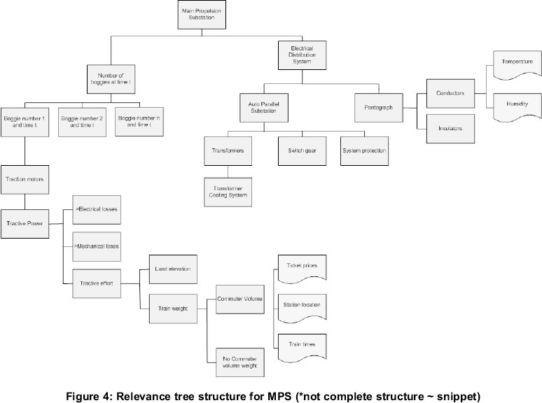
The demand was then modelled according to the source. This method provides less transparency but is more seamless. The physical system and components were first broken down. The method applied here was by first evaluating the main demand elements such as the electrical distribution system and commuter transit system and then have a breakdown of each element. The end result was a hierarchical structure that illustrates several levels of the subject matter. The concept is best known for technology assessment and the impacts of decision making and the sub impacts on lower branches of the hierarchy. The illustration of Figure 4 presents a basic structure (*incomplete) of the demands sourced from the main propulsion system. Two broad streams in the second level are presented, namely the elements of the commuter system (actual demand stemming from the boggies) and the train distribution system. Coincidentally, two simulation models were also used to model the train distribution system and the commuter system. Each branch is analysed until each section or entity is exhausted. The final elements in the model will present the cause and effect factors.
To better explain this, consider the following: The electrical distribution system is an element of the MPS. There are two components of an electrical distribution system, namely the auto parallel substations as compensatory measures to line loses and voltage drop and the pantograph used to supply electrical power to the commuter rail boggies. The last physical system may be resolved into a series of basic formulae. For the catenary, the resistivity is a dependent upon the temperature given by (ignoring reactive components):
![]()
Where:
α: Temperature coefficient of resistance
The cause and effect is hereby identified. As mentioned before, the ANN model hides the complexities of how the influential variable correlates onto the physical entity. Having a breakdown of each entity does not bare significance as much as the causes by which the physical parameters are altered. Most causes may be linked to more than one sub entity inside the relevance tree. Although the underlining factors or causes may be resolved to physical factors, this may not always possible. Some factors vary in accordance with social, economic and political factors. For instance, the tractive effort needed is significantly dependent on two factors, namely land elevation and train weight (see Figure 4).
The train weight may be further sub divided into the no demand weight and the demand weight. For the demand weight, the commuter volume (amount of passengers on the train) is a significant factor. The commuter volume is dependent on the time of day, train frequencies, station location, ticket prices and several other social factors. Irregularities in the commuter volume leads can be tracked for special days and holidays.
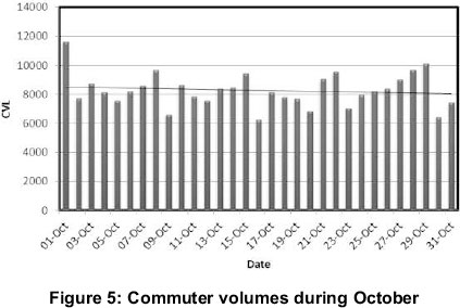
The commuter volume demand is not easily predictable since certain parameters that determine the commuter volume is difficult to determine, specifically social influences. The commuter volume demand was identified and was quantified by means of ticket collection vending machines.
Figure 5 illustrates the demand over a month and the linear trend. Special days such as weekends are easily identifiable by means of a drop in the commuter demand.
In the final model, this input vector is critical and is used as a correlation to the final demand. It is important to note that the relevance tree and modelling of physical factors may be further developed into a simulation model. The following methodology is recommended for the relevance tree breakdown model for the identification of elements for input vectors (ANN model):
i) Identify the highest level the hierarchy structure (demand or source). For a demand derived model, more data acquisition may be required. Data acquisition places constraints on the insertion of elements into the ANN model. All other elements are dependencies of this element. i.e. The MPS in this case.
ii) The top level hierarchy is broken down into elements. The modelling of the physical system is paramount in determining the elements. Once this is exhausted, elements are then broken down into first principles whereby the influential variables are identified. First principles refer to basic formulae that mathematically describe the physical parameters of the system. For example, force, losses, resistance, reactance, tractive force. This becomes critical since influential variables may easily be identified. For human dependent factors (carriage weight), social, political and economic factors apply. This may mostly be quantifiable in terms of trend analysis. The cause and effect terms how the demand will be influenced by these variables.
iii) Determine which 'causes' are quantifiable. This places constraints on the accuracy of the model. Each element bares a degree of significance. This is usually presented in weighted notation for an ANN model at time t. Dependent upon the significance of the influential variable and accuracy of the data acquisition, the effectiveness of the input vectors may be determined. In many time series models, elements that vary in small magnitude and that may be defined by the potential demand are omitted.
iv) Where possible, a trend analysis of data elements should be derived. This will assist with medium to long term forecast modelling. Each variable must be quantifiable by means of data acquisition or stochastic or deterministic trend analysis.
v) This data can now be inserted in vector form as input parameters into the ANN Model.
The following vectors were found to be quantifiable elements that suffice a short term demand forecast modelling of the MPS demand. This was based upon quantifiable model parameters identified in the relevance tree.
x1: Defines the input vector for the daily commuter volume
x2: Defines the input vector for the dry bulb temperature
x3: Defines the input vector for humidity
x4: Defines the input vector for past demand data x5: Defines the input vector type of day identification (special days, weekends). This also used in regression type models.
x6: Defines the input vector for time of day xn: Additional model parameters where n = 7,8,9...
Thereafter, a comparison between the factors identified by the simulation model and relevance tree was conducted. Usually elements are provided by various providers and a relevance tree model provides consumer specific model parameters.
4. Comparing elements found in the relevance tree to the simulation model
The vector summation of all variables may be further developed into a simulation model. The simulation model for the commuter rail system was divided into two models. One model simulated the boggie system whilst the second simulated the electrical distribution system. A simulation model may be considered as the mathematical derivation of the relevance tree. The demand may be summated to include all sub components and effecting factors. For this particular model, there were a few discrepancies between the elements identified in the simulation model and the elements identified in the relevance tree. This is due to elements having a minor impact on the final demand not being modelled or grouped into the potential demand. The simulation model did not also account for elements not easily quantifiable such as land elevation and varying commuter volumes. Hence, why an ANN based model accounting for these factors may prove to be more accurate. Finally the elements that account for noise are not easily identifiable or quantifiable. Several authors' present models whereby the noise may be define in a stochastic methodology.
5. Conclusion
This paper proposed a method of identifying input vectors for an ANN based forecasting model. Due to the rise in popularity of demand forecasting methods by means of artificial neural networks, the identification of input parameters are of paramount importance. Relevance tress may be used as identifying these input vectors by means of a graphical hierarchical structure. Then finally, the demand is resolved into mathematical models that define the physical properties of the demand. Thereafter, factors effecting the demand are resolved. This also makes the identification of nonphysical factors easier, such as economic, political and social factors.

More importantly are the quantification of the model input vectors which have been found to place constraints on the accuracy of the model.
The output model parameters for the ANN demand forecasting algorithm were identified by means of the consumer and supplier by means of the supply agreement. In this case, the correlation of these input vectors has to be resolved into the energy demand and NND. Thus far the comparison has been made in terms of a comparison between the simulation model and relevance tree model. The omission of certain elements may have been the cause of inaccurate data in the simulation model. However, in terms of the identification of quantifiable input vectors, the relevance tree model is recommended.
References
Alfares, H. K., & Nazeeruddin, M. (2002). Electric demand forecasting: literature survey and classification of methods. 33(1). [ Links ]
Bose, N. K., & Liang, P (1996). Neural network fundamentals with graphs, algorithms, and applications. McGraw-Hill. [ Links ]
Bosque, M. (2002). Understanding 99% of artificial neural networks. Writers club press. [ Links ]
El-Debeiky, S. M., Hasanien, N. E., & Kandil, M. S. (2002). Long-term demand forecasting for fast developing utility using a knowledge-based expert system. IEEE transactions on Power Systems, 491496. [ Links ]
El-Sharkawi, M. A., Marks, R. J., Atlas, L. E., & Damborg, M. J. (1991). Electric demand forecasting using an artificial neural network. IEEE transactions on Power Systems, 442-449. [ Links ]
Huang, S. R. (2002). Short-term demand forcasting using threshold autoregressive models. 144(5). [ Links ]
Liao, G.-C., & Tsao, T.-P (2004). Application of fuzzy neural networks and artificial intelligence for demand forecasting. Electric Power Systems Research. [ Links ]
Lisboa, P G. (1992). Neural Networks: Current Applications. Chapman & Hall. [ Links ]
Lotufo, A., & Minussi, C. (1999). International conferance on Electric Power Engineering. [ Links ]
Mediros, M. C., & Soares, L. J. (29-30 May, 2006). Robust Statistical Methods for Electricity Demand Forcasting. Paris: RTE-VT workshop. [ Links ]
Moghram, I., & Rahman, S. (October,1989). Analysis and Evaluation of Five Short-Term Demand Forcasting Techniques. 4(4). IEEE Transactions on Power Systems. [ Links ]
Porter, A. L. (2007). A Guidebook for technology assessment and impact analysis. University of Michigan: North Holland, 1980. [ Links ]
Ranaweera, D. K., Hubele, N. F, & Papalexopoulos, A. D. (1995). Nonlinear autoregressive integrated neural network model for short-term demand forecasting. IEEE Transactions on Power Systems. [ Links ]
Wang, P-Y., & Wang, G.-S. (1993). Power system demand forecasting with ann and fuzzy logic control. [ Links ]
Received 18 June 2012
Revised 28 February 2013

