TECHNICAL PAPER
http://dx.doi.org/10.17159/2309-8775/2023/v65n3a1

 

Revised Regional Maximum Flood (RMF) method and regionalisation

 

 

J A du Plessis; S Masule

Correspondence

 

 

---

ABSTRACT

South Africa receives an average annual rainfall of about 450 mm. Hydraulic structures are typically constructed to either store or manage the excess water resulting from runoff. These hydraulic structures are designed and evaluated to withstand a particular flood peak that can occur in its catchment area. Adequate flow or rainfall records may often not be available to enable a reliable flood estimation. In South Africa an empirical estimation method (the Regional Maximum Flood (RMF)) that utilises regional envelope curves to estimate the maximum observed flood peaks that can be expected in a region, is available. The RMF method adopted by Kovács in 1980, and revised in 1988, is robust and simple to use. The current research revisits the method as applicable to South Africa, and presents an update of the method, taking more than 30 years of additional data and a revised regionalisation approach into consideration. Numerous previous researchers evaluated the RMF method and concluded that the method needs to be updated. It was identified that recently observed flood peaks exceeded the existing RMF envelopes. It was further identified that the Kovács regionalisation process is inconsistent, and a revised regionalisation approach was proposed. The revised regionalisation resulted in 15 RMF K regions and their associated envelope curves. The new RMF K regions are smaller, with the highest K value equal to 5.8 and the lowest value 2.8. The recommended envelope curves were drawn 15% above the maximum observed flood peaks for each region, allowing for possible future climate impacts. The revised RMF envelope curves are considered to adequately represent the RMFs in South Africa and are therefore applicable for determining the expected maximum regional flood at any site in South Africa.

Keywords: Regional Maximum Flood (RMF), flood peaks, regionalisation, safety factor, flood zone, transition zone, storm zone

---

 

 

INTRODUCTION

South Africa has experienced significant floods, including the Laingsburg and southeastern Cape floods in 1981, floods from the cyclone Domoina in 1984, the KwaZulu-Natal floods in 1987, the Orange River Basin floods in 1988, and the Limpopo floods in 2000 (Görgens et al 2006). In addition, the Western Cape experienced flooding in 2005, and the Eastern Cape and Free State experienced flooding in 2011 (Smithers 2012). It is critical to understand the magnitude and recurrence interval of these extreme floods to plan, design and operate hydraulic structures. In South Africa the methods used to estimate these flood peaks are based on probabilistic, deterministic and/or empirical methods (Kovács 1988; Parak & Pegram 2006; Van der Spuy & Rademeyer 2010; Van Dijk et al 2013; Gericke & Du Plessis 2013). This research focused on the update of the RMF as one of the empirical methods, and presents an improved approach in developing a new set of regional curves, using an extended data set, for use to estimate maximum regional flood peaks as an upper limit value to be expected.

Estimation methods

Probabilistic, deterministic and empirical flood estimation methods were developed by various institutions from the late 1960s, using only data available at that time. These methods estimate flood peaks using either historical flood peaks or rainfall as the primary hydrological input data (Smithers 2012).

Probabilistic methods

Probabilistic methods estimate flood peaks by performing a flood frequency analysis of historically observed streamflow records, resulting in a direct estimation of flood peaks for various return period or exceedance probabilities. Their application is limited to catchments with suitable streamflow data (Van Dijk et al 2013). Probabilistic methods perform frequency analysis at a single specific site on observed streamflow data. The method assumes that the observed streamflow data comes from a known probability distribution and that it is stationary (Gericke & Du Plessis 2013). Beven (2000), cited by Smithers (2012), identified limitations associated with a direct probabilistic approach. It was identified that, while the actual distribution of flood peaks is unknown, numerous probability distributions may reasonably fit the plotted observed streamflow data, but when extrapolated, these result in significantly different estimations of flood peaks. Often, observed flood peak records are short, representing only a small population of the flood peaks at a given site. Additionally, while probabilistic methods presume that flood propagating variables are stationary, the statistics of data could have changed over the period of the recorded streamflow data. As a result, it ignores any changes in the runoff generating variables associated with incidents of greater magnitude.

Deterministic methods

Deterministic methods are used to estimate design period flood peaks and the expected maximum flood peaks, denoted as the Probable Maximum Flood (PMF). Deterministic methods suppose that the probability of the resulting flood peak and PMF occurring in any year depends on the probability of the causative rainfall. This is because it is assumed that the frequency of the determined flood peak and the causative rainfall are assumed to be equal, at the same time being influenced by catchment characteristics and model parameters (Smithers 2012). These methods, however, have shortcomings that impact significantly on the anticipated flood peaks. The disadvantages are that they rely on yet-to-be-verified hypotheses (translated into numerical parameter values such as runoff reduction factors) and rainfall coefficients such as storm rainfall area reduction factors, the transition between storm and storm losses, and the validity of unit hydrograph principles in the presence of significant flooding (Van der Spuy & Rademeyer 2010).

Empirical methods

Empirical methods are calibrated using streamflow data from hydrologically comparable sites in order to generate a regional

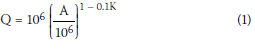
flood frequency curve that is appropriate throughout the region (Smithers 2012). Empirical methods should be utilised exclusively in their calibrated catchments (Van Dijk et al 2013; Gericke & Du Plessis 2013). Empirical methods use a regional approach, which is generally preferred over the at-site frequency analysis (Kjeldsen et al 2002), as it employs data from multiple catchment sites. Kachroo et al (2000) stated that a regionally based analysis provides a complete representation of historical flow data from a homogeneous region. A number of authors (e.g. Cordery & Pilgrim 2000; Nortje 2010; Gericke & Du Plessis 2013; Nobert et al 2014) recommended the use of regionalised methods, as these have benefits over site-specific methods using short records. Van der Spuy and Rademeyer (2010) defined empirical approaches as methods "based on observation or experience rather than theory or pure logic", in which flood peak frequencies are estimated using mathematical models established through the analysis of existing streamflow data. According to Wang (2000), the methods are based on the concept of transferring hydrological data from sites located in a homogeneous region to sites with little or no historically observed data. Homogeneous regions are established through regionalisation, which enables the selection of a frequency distribution or envelope curve that is suited for a specific region (Kachroo et al 2000). The RMF is one such empirical method. The method was adopted from Francou and Rodier (1967) by Kovács (1980) for South Africa. Francou and Rodier (1967) identified three zones that define the method, namely storm, transition and flood zones (Figure 1). The flood zone is governed by Equation 1.

 

 

 

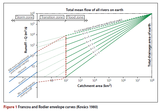
Where:

Q = discharge (m³/s)

A = catchment area (km²)

K = Francou and Rodier regional coefficient.

The RMF method estimates flood peaks using flood envelopes in homogeneous regions, and it is empirically established for obtaining extreme floods that represent the expected upper realistic limit in a region (Kovács 1988). Furthermore, it is used to calculate the Safety Evaluation Discharge (SED), a level pool peak discharge used to determine the associated safety risk for a spillway system of a new or existing dam in the event of an extreme flood, in accordance with the SANCOLD (South African National Committee on Large Dams) guidelines (SANCOLD 1990). The RMF is also extensively used by practitioners, and specifically the Department of Water and Sanitation, as a guiding upper limit flood peak estimate when comparing different estimated flood peaks, using different approaches. This research does not investigate the applicability of the method, but builds on the well-established use thereof in South Africa and since the method was last updated in 1988 (making available more than 30 years of additional data for further analysis), focusing on the improvement of the RMF method for use in South Africa.

Several reviews on the 1988 RMF method have been conducted, and Pilon and Adamoski (1992), cited by Smithers (2012), acclaim the method for its ability to estimate floods (regional maximum floods and design flood peaks associated with a specific recurrence interval (RI)) in the absence of streamflow data. Pegram and Parak (2004) stated that the RMF method is a robust and simple-to-use method that estimates maximum regional flood at any site of interest by considering only the regional envelope and catchment area. However, various other studies have expressed and highlighted concerns and inconsistencies with the method. Görgens (2007) asserted that flood peaks that occurred after 1988 might have surpassed the RMF envelopes. Van Vuuren et al (2013) stated that the Kovács 1988 analysis of the RMF should be reviewed by including all the available and applicable data to verify and/or reproduce the maximum envelope curves. Smithers (2012) stated that the Kovács (1988) RMF regions must be updated and refined due to the availability of additional data. He further added that it would be prudent to investigate the use of probability of exceedance associated with the RMF. Verwey (2015) stated that Kovács's method of regionalisation is inconsistent. Verwey (2015) then investigated a new approach that incorporates a safety factor into the individual K values per station prior to regionalising them into distinct regions. Kovács (1980; 1988) added a safety factor AK to the K value that was already regionalised. Verwey (2015) argued that the added AK has no mathematical or scientific basis for its values. This argument was made in light of Kovács's (1980; 1988) omission of a mathematical or statistical explanation for AK. As a result, Verwey (2015), and subsequently Swanepoel (2017), developed a statistically sounder new safety factor (AQ), applicable to station flood peaks, before regionalisation. Du Plessis and Masule (2023) evaluated the methodology used by the Kovács 1988 RMF method, and concluded that the method needed to be reviewed, given various inconsistencies with the data used by Kovács (1988), and the observation that some of his RMF values had already been exceeded by recent observed flood peaks.

Regionalisation

New safety factor approach for régionalisation

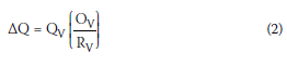
Verwey (2015) proposed a methodology based on the addition of a calculated ∆Q to each station's largest historical observed flood peak (Q₁), taking into consideration that not all stations used in the analysis have the same record length or span the same period of analysis. For each station, the method results in a new station flood peak (Qs). By substituting the Qs value and the corresponding area into the Francou and Rodier (1967) flood zone equation (Equation 1), a new calculated K station value (K_S) is obtained. The AQ is composed of three parameters (Ov, Rv and Qv) that account for the statistical characteristics of each gauging station's Annual Maximum Series (AMS) prior to regionalisation, as illustrated in Equation 2 (Verwey 2015).

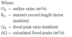
The Ov (outlier value) factor (Equation 3) takes into consideration whether or not the station's highest recorded flood peak Q₁ is an outlier value.

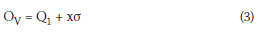
The value of Q₁ is considered an outlier if it proves to be greater than the value associated with the outlier threshold determined by the adjusted boxplot outlier test using the AMS.

The factor adjusts Q_x based on its outlier status; if an outlier is observed, one standard deviation (x = 1, therefore 0) is added to Qi alternatively, two standard deviations (20) are added.

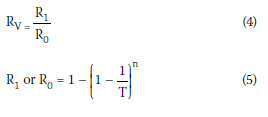
The R_v (station's record length) factor (Equation 4) was introduced to account for the gauging stations' varying record lengths. The Rv is expressed as the ratio of the probability (Ri) of a T-year flood occurring within the available record length (n) of the station to the hydrological risk (R₀) (that a T-year flood will occur in T years) (Equation 5) (Swanepoel 2017).

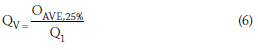
The Qv (flood peak ratio) factor (Equation 6) was added to scale the station's highest observed flood peak (Q₁) to the average of the station's top 25% of flood peaks (referred to as Qave 25%) (Swanepoel 2017).

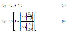
The Qs values can then be determined using Equation 7, and subsequently Ks values using Equation 8, rewritten from Francou and Rodier's (1967) flood zone equation.

The K_S values are then used to regionalise flood peaks, and with the addition of superimposed catchment variables, an RMF K regional map of homogeneous flood regions can be delineated.

Catchment variables for régionalisation

Agarwal et al (2016), Rosli et al (2019) and Ahani et al (2020) all defined regionalisation as the process of transferring hydrologic information from gauged catchments to ungauged catchments with similar characteristics, thereby forming homogeneous regions. Their similarities are determined by their geographical proximity and shared hydrologic characteristics and other defining variables. Catchments identified as similar are combined into a single region. Numerous studies assessed regionalisation approaches for delineating homogeneous flood regions. The Groupe de recherche en hydroclimatologie statistique (GREHYS 1996) investigated four distinct approaches: region of influence (ROI), canonical correlation analysis, cluster analysis and L-moments statistics. Parajka et al (2005) compared four approaches in a similar manner: the ROI, spatial proximity, catchment variables and flood moments (probability weighted moments and L-moments). The catchment variable approach is based on catchment characteristics and does not include complex site statistics, and is suited for regionalisation studies that are based on an empirical nature (Ahani et al 2020). Ahani et al (2020) defined catchment variables as physiographic, meteorological, geological, geographic location, soil type and land use. Spatial proximity and physical similarity that consider catchment variables, are two methods that have been implemented through models and software applications to establish homogeneous regions. The two methods are implemented differently based on the catchment-level assumptions. A potentially hydrologically homogeneous region would then be identified as catchments with similar variables, and at-site statistics are then used to independently assess if the region is homogeneous. It is urged that, despite the variety of approaches to regionalisation, a careful selection of variables affecting rainfall runoff is necessary to effectively distinguish runoff behaviours within a region (Zhang & Stadnyk 2020).

Van Dijk et al (2013) identified three variables that have a cumulative effect on a region's potential runoff response: climatic, physiographic and topographic. Benson (1964) identified climatic and catchment characteristics (catchment size, vegetation, land use/cover and soil type) as the critical hydrological variables affecting runoff.

 

STUDY AREA

The study area applicable to this research is limited to the national boundaries of South Africa and uses data obtained from the Department of Water and Sanitation (DWS) flow gauging stations (which include dams) and the South African Weather Service (SAWS) rainfall gauging stations located within the study area. The dam station data presents calibrated (routed) dam inflow data, which includes the maximum flood peaks for South Africa's major dams. The river flow station data reflects the data recorded at river gauges.

Data sources

Flood data

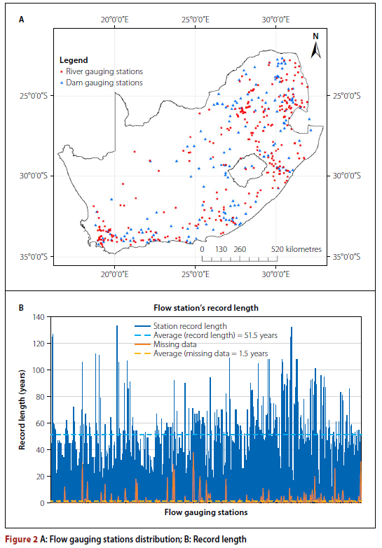
The DWS provided the Annual Maximum Series (AMS) of 494 stations, comprising 316 river gauging stations and 178 dam stations. The locations of the gauging stations and their record lengths are depicted in Figure 2 on page 4.

 

 

Rainfall data

Two rainfall data sets were used in the research:

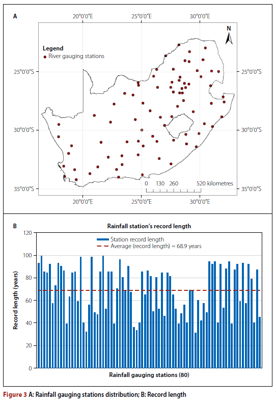
1. Design rainfall from Smithers and Schulze's (2002a) Design Rainfall software dataset

Seven-day 1:100-year storm rainfall data of 80 rainfall stations (Figure 3 on page 5) with a reasonably even distribution, chosen in accordance with the South African Weather Service's Rainfall Stations Reference Grid, was extracted from the Design Rainfall software. Alexander (2006) stated that extreme flood peaks are the result of prolonged and widespread extreme rainfall events such as the 7-day rainfall. The 7-day rainfall was significant in establishing rainfall isohyets that assisted in the regionalisation process.

 

 

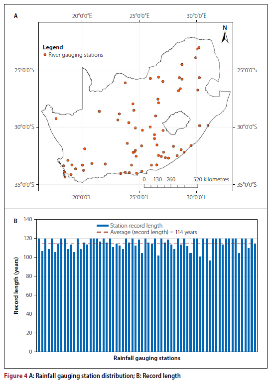
2. Daily rainfall from the SAWS and Lynch dataset

A consolidated dataset of one-day rainfall from SAWS and Lynch was created (Figure 4). SAWS provided data from 69 gauging stations, and much older data of 35 gauging stations was extracted from the Lynch database. The gauging stations had an average record length of 114 years. The Lynch database provides data from a spatial database of daily rainfall in South Africa. The one-day rainfall data was required to determine the 15-minute rainfall intensities that enable the determination of point discharge at the storm zone. The 15-minute rainfall data was scaled down from one-day annual maximum series rainfall using Smithers and Schulze (2002a) scaling factors.

 

 

METHODOLOGY

This section provides the detailed methodology that was followed during the research to update the 1988 RMF approach.

Updating of the 1988 RMF method

Database of maximum flood peaks

In compiling the observed flood peak database the principles were (i) that only the Annual Maximum Series (AMS) from the DWS dataset would be used, and (ii) that at any one gauging station only the maximum observed flood peak would be selected. A new database, containing 494 flood peaks was then created.

Determination of Q_S and K_S values

Prior to regionalisation, using the AMS of each gauging station, the statistical parameters utilised in calculating AQ were determined, and AQ was calculated using Equation 2. The Q_S values were determined using Equation 7, which were then used to calculate the K_S values using Equation 8.

The K_S values were then regionalised to determine a grouping of Ks regions with similar K_S values, and subsequently delineating final RMF K regions by incorporating various geographical, climatic and relief variables.

Régionalisation

Flood zone

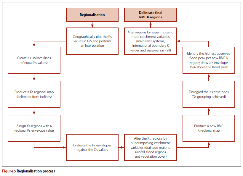
Regionalisation makes it possible to transfer data from gauged catchments to similar ungauged catchments in homogeneous regions. The regionalisation process is illustrated in Figure 5, and explained in more detail in the following paragraphs.

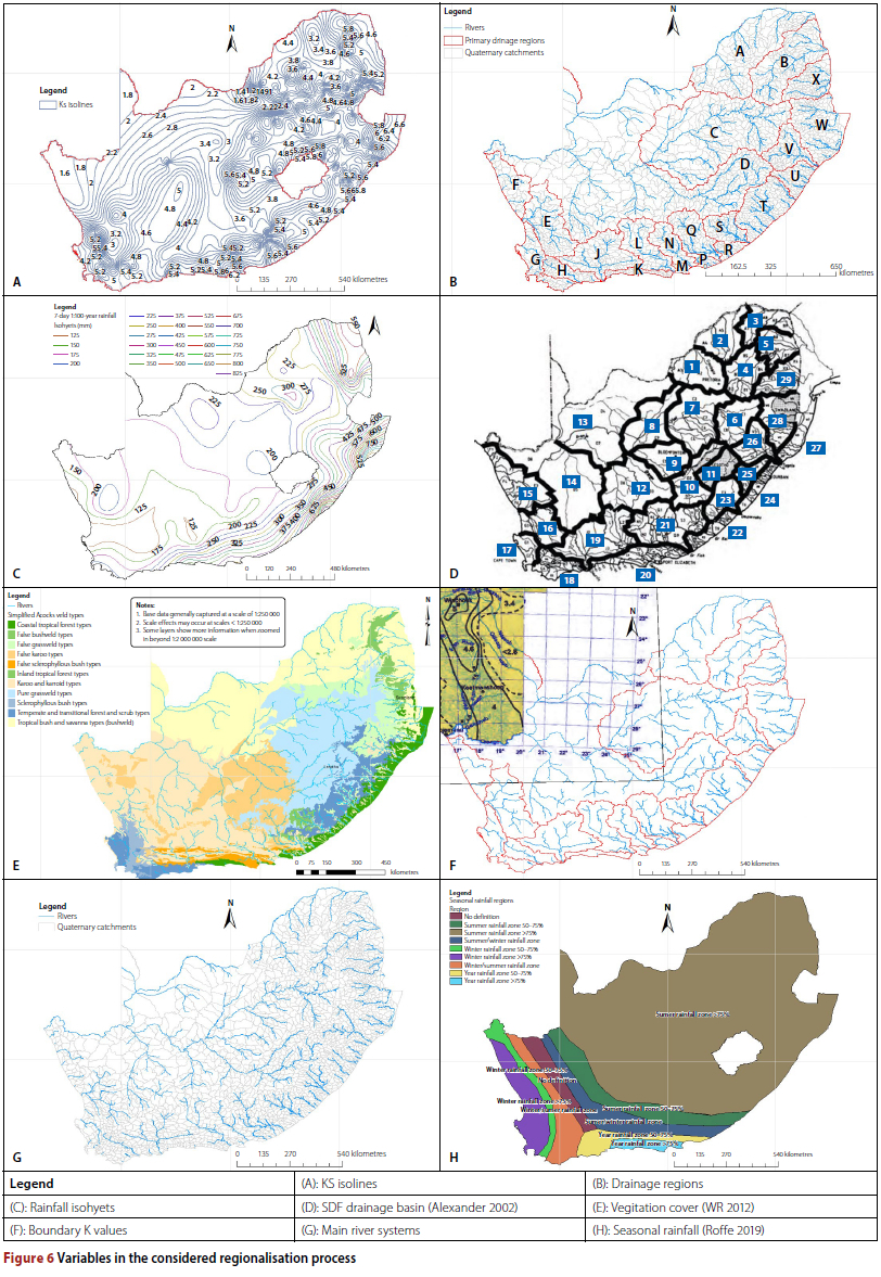
Several variables were superimposed in delineating the RMF K regions. The variables were superimposed sequentially from the most influential to the least. These were the K_S (stations calculated K-value) values, drainage regions, rainfall pattern, flood homogeneous regions (SDF, Veld Types, and RMF regions), vegetation and soil type, K values at international boundaries (Regional Maximum Flood envelopes lines Ke value), river systems and seasonal rainfall regions. These variables are shown in Figure 6, and can be expanded on as follows:

■ K_s values (Figure 6A):

The K_S isolines were regarded as the most influential variables in determining the new RMF regions. The K_S values were plotted geographically in GIS and spatially interpolated to generate K_S iso-lines (Figure 6A). K_S regions were then directly drawn from the isolines. The K_S regions were used to group gauging stations with similar K_S values, without any influences from other variables. As a result, 15 Ks regions were delineated. A regional K_S value was assigned to each region and a representative envelope curve was drawn. It should be noted that no objective criterion was used in selecting the regional K_S envelope value used, but a base value of K = 1.8 with a 0.2 interval was chosen based on Kovács's original approach. As a result of the selected interval, a grouping of multiple Ks isolines was required to delineate a single Ks region. It was then necessary to graphically depict the assigned regional Ks envelopes against the Qs values of stations in each Ks region. To further improve the regionalised 15 K_s regions to achieve a grouping of gauging stations with Q_s values not exceeding and not significantly plotting below the assigned regional K_s envelopes, the K_s regions were adjusted by including the influence of physiographic and climatic variables as outlined below.

■ Drainage regions and topography (Figure 6B):

It was anticipated that the regionalisation of the K_s regions could be improved by reflecting the quaternary catchments of south Africa. The quaternary catchments (1946 catchments), along with the topography, were superimposed to provide guidance regarding the edges of the flat areas and areas of small catchments.

■ Rainfall (Figure 6C):

The 7-day 1:100-year rainfall isohyets were superimposed on the K_s regions, and the K_s regional boundary was then adjusted to follow the isohyets where few or no K_s values were available.

^■ Flood homogeneous regions (Figure 6D): Three of south Africa's well-established flood regional maps that are used for local practices in flood hydrology were superimposed in the adjustment of the K_s regions. These include the standard Design Flood (sDF), the General veld Types and the 1988 RMF regions. The eastern escarpment consists of numerous small catchment areas, therefore the flood homogeneous regional boundaries provided guidance for the RMF regional boundaries to follow.

■ Vegetation and soil (Figure 6E):

Vegetation and soil types are landscape characteristics that interact at a catchment scale with climate characteristics such as rainfall to produce catchment runoff. Vegetation and soil types were superimposed in altering K_S regions. It was found, however, that the already adjusted K_S regions correspond well with the vegetation and soil type boundaries. This was because vegetation and soil boundaries are closely linked to the topography.

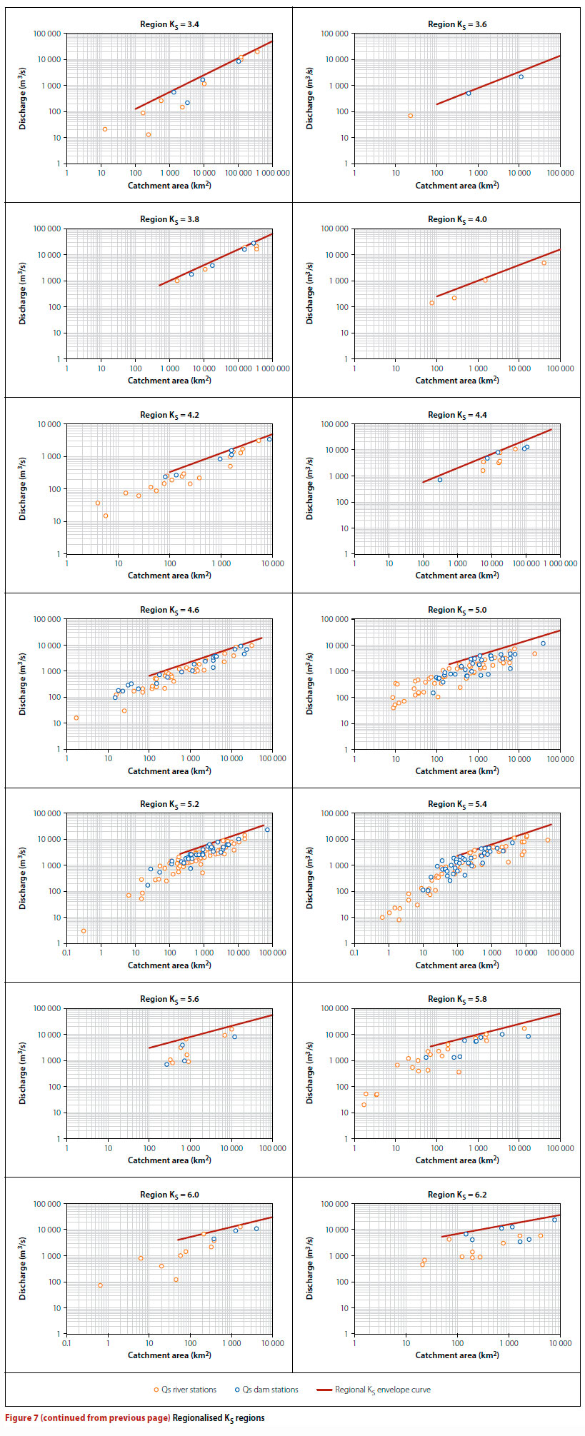
The adjusted K_S regions were graphically analysed, plotting the Q_S values against the K_S envelopes. It was then concluded that regionalisation had been achieved, as depicted in Figure 7. Based on the results presented in Figure 7, the systematically adjusted regionalisation was deemed to be completed. As a result, 15 regions were subsequently delineated. At this point, the Q_S values of each station and the regional K_S envelope curves were disregarded (regionalisation using Q_S had been completed) and consideration was now given to the actual observed flood peaks Q₁. Note that the K_S values were only used for regionalisation.

The RMF K regions were further enhanced as follows:

■ K values along international boundaries (Figure 6F):

Boundaries of the RMF K regions where few or no Kg values were available, followed the rainfall isohyets. However, along the borders of south Africa and Namibia where, over a large area, no K_s values were available, the updated RMF regions of Namibia from Cloete et al (2014) were georeferenced and superimposed to adjust the boundaries of the K regions to be consistent with the K values for Namibia.

^■ Rivers (Figure 6G):

Major rivers were superimposed to better understand the fluvial landscape, with an emphasis on the flow direction and length of the river from its catchment boundary to the gauging station.

^■ Seasonal rainfall (Figure 6H): Rainfall in south Africa is caused by a variety of weather phenomena that occur in different regions and at different times of the year. The seasonal rainfall distributions were similarly superimposed. The boundaries of the all-year rainfall zones and the winter rainfall zones were used to justify several delineated final regions.

■ River K values:

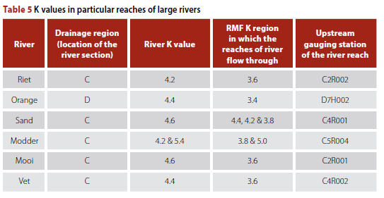
Kovács (1988) stated that rivers that flow through multiple RMF regions may exhibit distinct flood characteristics that differ significantly from those found in the delineated K region, thus the lower reaches of these rivers have a different K value compared to that of their upper reaches. The rivers were investigated and the sections with a different K value were identified.

Storm zone

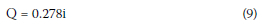
In the storm zone, the peak discharges depend only on rainfall intensity. For a catchment area of 1 km² the discharge is as presented in Equation 9, where i is the maximum 15-minute rainfall intensity in mm/h. Kovács (1988) stated that a 15-minute period is the approximate time of concentration in a catchment of 1 km².

To determine the required regional discharge at the storm zone, the 15-minute rainfall intensities were calculated from 15 minutes of rainfall, scaled from the 1-day rainfall, using smithers and schulze (2002b) scaling factors. The rainfall stations used in this analysis were selected from catchment areas where the peak discharges depended only on rainfall intensity. Flow gauging stations in these catchment areas had recorded extreme flood peaks. The selected rainfall stations were then geographically located using GIs. For each station a predetermined cluster group and the corresponding scaling factors according to smithers and schulze (2002b) were identified. smithers and schulze (2002b) presented ratios of 24-hour:1-day rainfall values corresponding to each cluster group which included an average, median and standard error. The ratios are presented in Table 1.

 

 

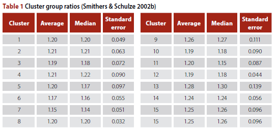
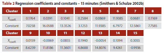
The median ratios were used to convert the highest 1-day rainfall values (selected from the annual maximum series dataset of each rainfall station) to 24-hour rainfall values. The required short duration (15-minute) rainfall values were then scaled down from the 24-hour scaled rainfall, using the regression coefficients and regression constants in Table 2, as presented by smithers and schulze (2002b), of each corresponding cluster group.

 

 

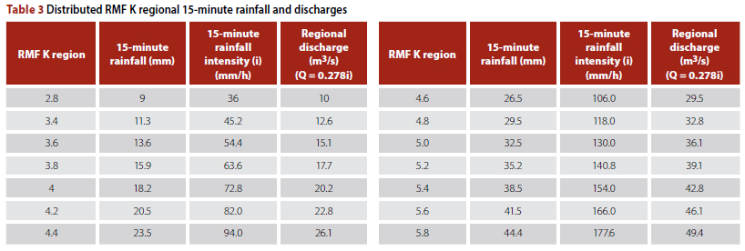
A regional 15-minute rainfall was then selected as the highest 15-minutes rainfall of all gauging stations in each RMF K region. The regional 15-minutes rainfall was converted into rainfall intensities (mm/h). The 15-minute regional rainfall intensities were substituted into storm zone Equation 9 to determine the regional discharge for a 1 km² catchment. These regional discharges are presented in Table 3 on page 11.

When the regional discharges for the storm zone in Table 3 were compared to the Kovács 1988 regional discharges, it was observed that Kovács's regional discharges were significantly larger. There is, however, no documented reference to where Kovács obtained his data from, and the data in Table 3 was therefore adopted, being the best available information. The available observed flood peaks from gauging stations used in this research with catchment areas approximately 1 km² in size were, however, all significantly lower than the flood peaks based on the flood zone equation, providing justification for the decision to adopt the values from Table 3.

Transition zone

No regionalisation was carried out in the transition zone, but only the determination of envelope curves. The transition zone envelope curves provide a smooth transition between the storm and flood zones. To determine the transition zone envelope curves, the regional discharge associated with 15-minute rainfall intensity at the storm zone, as determined in Table 3, and the RMF K envelope curve in the flood zone were required.

Homogeneity of the RMF K regions

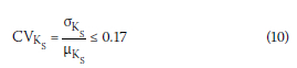
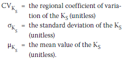
Due to the numerous adjustments, the homogeneity of the newly established RMF K regions was investigated. The homogeneity of RMF K regions was determined using a statistical approach where a coefficient of variation (CV) was calculated for each RMF K region and then compared to a CV threshold, adopted from Kovács (1980). The purpose of this evaluation was to assess the dispersion of K_S values within a region. The K_S values were used since they were the primary parameters in the regionalisation process. Kovács (1980) calculated the CV of his Kr values to determine the homogeneity of his 1980 RMF flood regions. According to Kovács, a CV of less than or equal to 17% satisfied the fundamental requirement of regionalisation and that of homogeneous regions. Based on his finding, the homogeneity of each RMF K region was evaluated against a maximum CV value of 17%. The CV was tested, using Equation 10.

Determination of envelope curves

The regional envelope curves were developed for the flood zone and the transition zone.

Flood zone

The envelope curve in the flood zone was established by considering the regional boundaries of the RMF K regions, identifying the separation between the flood zone and the transition zone, and furthermore by plotting flood peaks against respective catchment areas and drawing the K envelopes 15% above the highest observed flood peaks (Q₁) in each K region. These were carried out after regionalisation. The highest observed flood peak ("envelope determining flood peak") in each K region was identified, from which the regional K envelope was then drawn 15% above the selected flood peak value. The 15% was adopted from Kovács (1988), and deemed as the safety factor above the highest selected flood peak. The Kovács 1980 envelope curves, which were drawn above the regional maximum flood peak, were in most cases between AK = 0.2 to AK = 0.31 above the maximum observed value, which is equivalent to an increase in discharge of between 15% to 30%, depending on the catchment area. Therefore, in the flood zones for all K regions, the K envelope curves were drawn by adding AK = 0.2, which is 15% of the flood peak. The assigned regional K envelope values were from < 2.8, 2.8, 3.4 to 5.8 with a 0.2 increment. The boundary between the flood zone and the transition zone (still to be discussed) was identified as being at the catchment area where the trend of the plotted observed flood peaks changes from aligning with the direction of the flood zone envelope curve.

Transition zone

The envelope curves in the transition zone were drawn between the storm zone and the flood zone. The envelope was drawn from the discharge associated with the 15-minute duration rainfall over 1 km² at the storm zone to the K envelope curve in the flood zone.

Return period of the RMF

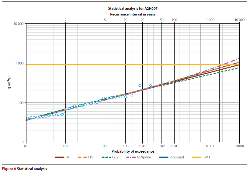
Kovács estimated the return period of the RMF to be 200 years (Kovács 1988). To assess this finding, the return period of the newly determined RMF values at 452 of the gauging stations in the DWS dataset were determined. The AMS of each gauging station was arranged in a descending order and a plotting position of each value was determined using the Cunnane formular. Cunnane was used as it is the suggested and the preferred plotting position in the DWS (Van der Spuy & Rademeyer 2010). The values were then plotted against the probability of occurrence on a log-probability scale, and the best visually fitting probability distribution selected.

The required probability of occurrence (hence return period) for a specific RMF was then determined as shown in Figure 8 on page 12 for station A2H007.

 

RESULTS

RMF K regions

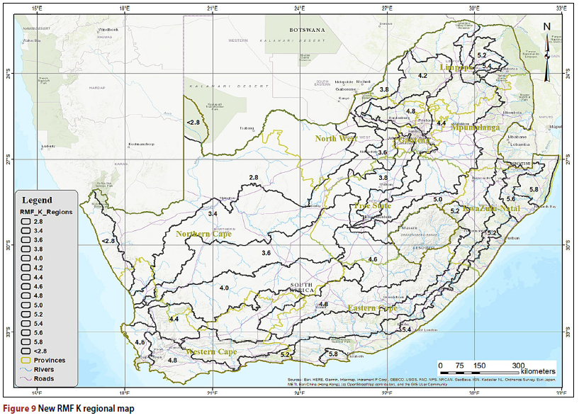
The regionalisation process resulted in the delineation of 15 RMF regions as presented in Figure 9 on page 12.

The RMF K regions with higher K values are dominated by hilly to mountainous relief, higher rainfall and smaller catchment areas. RMF K regions with lower K values are dominated by flat relief, lower rainfall and larger catchment areas. Similar trends were observed in the Kovács 1988 RMF regional map. The highest K region of 5.8 was delineated for the new RMF K regions, which was delineated to accommodate the gauging station that had exceeded the Kovács K_E Regions 5.4 and 5.6, with the latter the highest K region as defined by Kovács. The lowest K region represents a region with K values lower than K = 2.8; however, in accordance with Kovács (1988), such a K region was defined as < 2.8. Kovács (1988) stated that the RMF in such a region should be determined using a K value of 2.8.

When the RMF K regions (Figure 10A on page 13) were compared to Kovács's 1988 RMF regions (Figure 10B), general similarities and differences were observed.

 

 

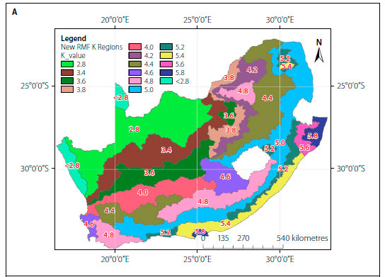
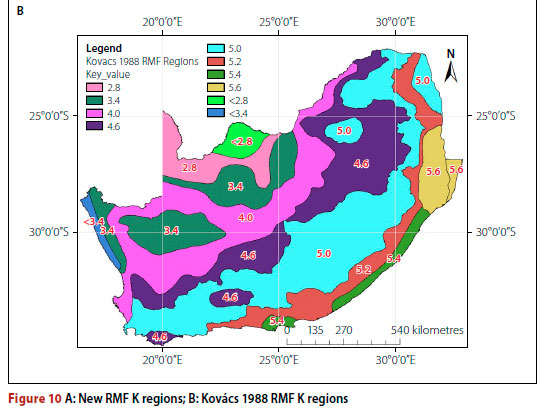
The new RMF K regional map showed that, in contrast to the Kovács 1988 RMF regional map, a more localised regional map, with regions having smaller areas, particularly those with high K values, was delineated. However, various boundaries of the new RMF K regional map corresponded to those of the Kovács 1988 RMF regional boundaries, and these were observed mostly in the western and northeastern parts of the country. The lower (2.8, 3.4) and the higher (5.0, 5.2, 5.4) K regions were observed to be consistent with those defined by Kovács, despite having different sizes. The high correlation and similarities between the new RMF and the Kovács 1988 RMF regions instil confidence in the validity of the new RMF regions. The new regions were delineated using a much larger dataset and longer record length compared to the Kovács 1988 regions. As a result, 15 RMF K regions were delineated in this study compared to Kovács's previous 8 RMF regions.

With the much larger dataset it was required to evaluate the homogeneity of the RMF K regions.

The homogeneity of the RMF K regions was evaluated using the statistical parameters (0 and µ) listed in Table 4 on page 14. The number of gauging stations located within a region are shown. Equation 10 was then used to calculate the regional coefficient of variation.

 

 

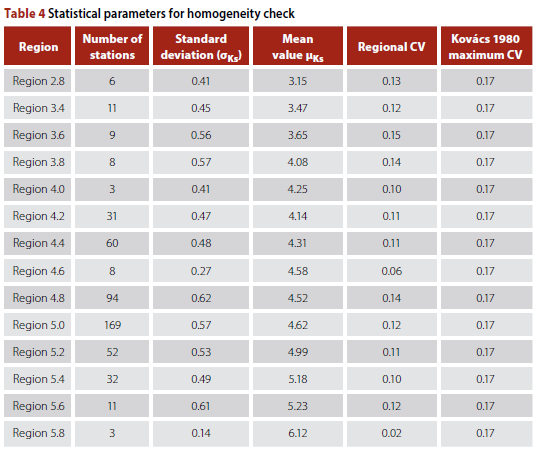
K regions 4.4, 4.8, 5.0 and 5.2 all had more than 50 gauging stations per region and, according to Table 4, a Cv of less than 0.14, which gave credence to the regionalisation approach. Based on the CV of the K_s values in each new RMF K regions, as discussed above, the regions were deemed to be homogeneous.

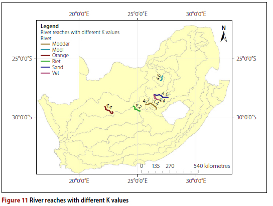
It was, however, observed that certain reaches of rivers running through the RMF K regional boundaries had a markedly different K value compared to the K value of the region, similar to what was observed by Kovács. The positions of these river reaches are shown in Figure 11 on page 14. If any flood estimation had to be carried out within these six reaches, a river K value different to the RMF K region in which it is situated needs to be used. The river reach K values and corresponding information are presented in Table 5 on page 14.

 

 

 

 

Envelope curves

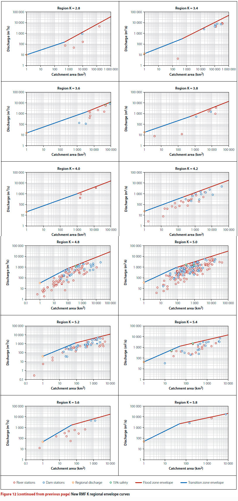
The final regional K envelope curves are presented in Figure 12.

The regional discharge at the storm zone increases as the RMF K values increase. The transition zone envelope was drawn from the regional point discharge to the regional K envelope curve in the flood zone.

In several RMF K regions the boundary between the flood zone and transition could not easily be defined due to the irregular and scatter plotting of the limited available observed flood peaks or a lack of gauging stations. In this regard, the transition zone envelope curves were drawn in the context of the Kovács RMF envelope curves where the largest catchment area

boundary of 500 km² was adopted. This was applied for RMF K regions 2.8, 3.4, 3.6, 3.8 and 4.0. In regions 3.6, 3.8, 4.2 and 4.6 a clear boundary between the flood zone and transition zone could be defined.

The storm zone regional discharges at 1 km² on the RMF K regional envelope diagram were significantly lower than those in the Kovács (1988) RMF. However, the regional discharges for the storm zone determined in this study were found to be significantly higher than the observed flood peaks for gauging stations plotting closer to 1 km². This finding confirmed that the regional 15-minute rainfall intensities used were indeed applicable.

It was observed that, for the higher K regions, most of the plotted maximum observed flood peaks in the flood zone follow the trend of the K regional envelope fairly well. The flood peaks plotting towards the lower limit of the transition zone were observed to be significantly lower than the storm zone regional discharge at 1 km². This provided confidence that the determined regional discharge at the storm zone associated with 15-minute rainfall intensity at 1 km² is applicable, even though these values are significantly lower than the Kovács storm zone values.

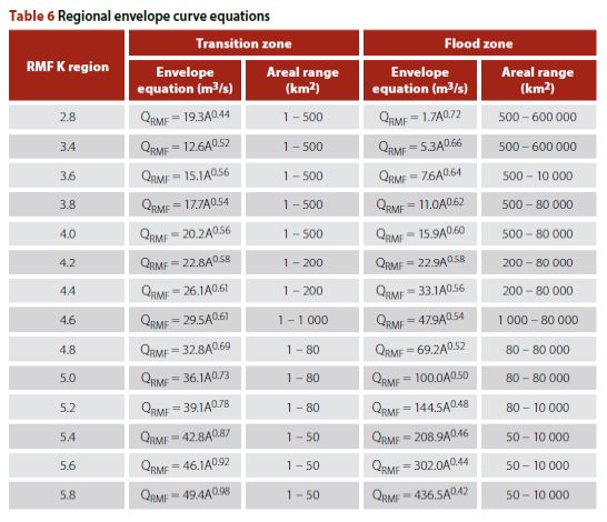
Envelope equations

The derived RMF K regional envelope equations are presented in Table 6 on page 17 along with their applicable catchment area range. The envelope curve represents the RMF that can be expected in each of the K regions for any catchment size. The applicable areal range corresponds to the catchment area boundaries of zones on the envelope curve diagrams in Figure 12. The applicable area range in the transition zone is defined by the catchment area from the storm zone to the flood zone.

 

 

Return period of the RMF

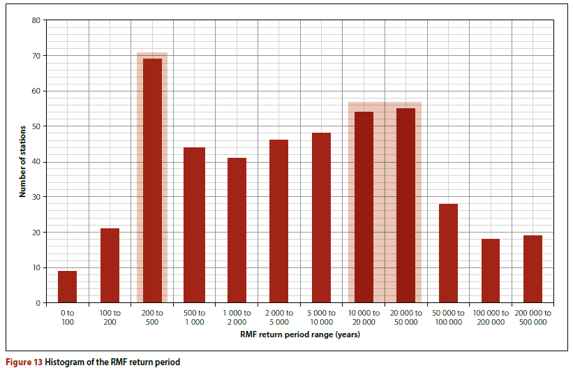
It was noted that the RMF values of gauging stations in a K region did not provide a consistent return period, but varied depending on the historical flood peaks and the catchment area. In the further analysis of the return period of the RMF, the stations (14 stations) with a return period of greater than 1 in 500 000 years were stations with very limited data or short record lengths and were therefore excluded from the analysis. Figure 13 on page 17 is a histogram of the number of gauging stations with RMF falling in various ranges of return periods.

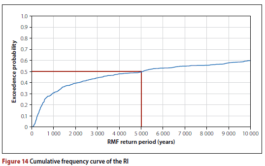
Figure 13 shows that 69 out of 466 stations had RMF values associated with a return period in the range of 200 to 500 years, while 109 stations were in the range of 10 000 to 50 000 years (both scenarios respectively highlighted by boxes in the figure). Most of the RMF values were associated with return periods greater than 1 in 2 000 years. A cumulative frequency diagram generated from the histogram in Figure 13 is shown in Figure 14. From Figure 14 it was observed that, for an exceedance probability of 0.5 (the median value), the return period associated with the RMF is 5 000 years.

 

 

Application of the RMF

To calculate the RMF of a site of interest, the RMF K regional map in Figure 9 and the RMF K regional envelope equations in Table 6 are used. This requires the following actions:

^■ The geographical location and catchment area of the sites of interest must be determined.

^■ The RMF K region of the site must be identified from Figure 9.

^■ The RMF K regional envelope equation must be identified from Table 6, corresponding to the identified RMF K region. It should also be remembered to identify the zone (transition or flood) of the site, using its catchment area.

■ Lastly, the required RMF should be calculated, using the identified RMF K regional equation for the correct zone, by substituting the catchment area of the site in the relevant equation.

^■ If the required RMF is for a site located along the identified river section with a different K value from that of the RMF K region, the RMF K regional envelope curve equation corresponding to the K value of the river section (see Table 5) should be used.

 

CONCLUSIONS

The objectives of this study were to develop an improved approach to estimate the RMF as an upper limit flood. A refined regionalisation approach was used to regionalise flood peaks, and 15 RMF K regions with their associated envelope curves were identified. The lowest RMF K region is 2.8 and the highest RMF K region is 5.8. The homogeneity of the regions was evaluated, and it was concluded that the regions were indeed homogeneous. The envelope curves in the flood zone corresponding to the RMF K regions were drawn 15% above the maximum observed flood peak. The transition zone envelope curves were drawn from the K envelope curve in the flood zone to the regional point discharge at 1 km² in the storm zone. It was evident from this study that the regional discharge associated with a 15-minute rainfall intensity at 1 km² was higher than the observed flood peaks that plotted closest to the 1 km² catchment areas. This supported the regional discharges at the storm zone. Envelope equations were generated for each region, which can be applied in estimating the RMF for any site of interest. It was concluded that the return period associated with median RMF peaks in this study was estimated to be 1:5 000 years, but ranged from less than 100 to more than 500 000 years, as opposed to the original Kovács estimation of 1:200 years.

 

REFERENCES

Agarwal, A, Maheswaran, R, Sehgal, V, Khosa, R, Sivakumar, B & Bernhofer, C 2016. Hydrologic regionalization using wavelet-based multiscale entropy method. Journal of Hydrology, 53(8): 22-32.         [ Links ]

Ahani, A, Nadoushani, S S M, Moridi, A 2020. Regionalization of watersheds by finite mixture models. Journal of Hydrology, 583: 124620.         [ Links ]

Alexander, W J R 2002. The standard design flood. Journal of the South African Institution of Civil Engineering, 44(1): 26-30.         [ Links ]

Alexander, W J R 2006. Climate change and its consequences - An African Perspective. Technical Report: University of Pretoria.         [ Links ]

Benson, M A 1964. Factors Affecting the Occurrence of Floods in the Southwest. Washington DC: United States Government Printing Office.         [ Links ]

Cloete, G C, Basson, G R & Sinske, S A 2014. Revision of Regional Maximum Flood (RMF) estimation in Namibia. Water SA, 40(3): 535-548.         [ Links ]

Cordery, I & Pilgrim, D H 2000. The state of the art of flood prediction. In Parker, D J (Ed). Floods. Vol II. London: Routledge, 185-197.         [ Links ]

Du Plessis, J A & Masule, S 2023. Evaluation of Kovács 1988 Regional Maximum Flood 556 Method. Journal of the South African Institution of Civil Engineering, 65(1): 35-44.         [ Links ]

Francou, J & Rodier, J A 1967. Essai de classification des crues maximales observées dans le monde. Cahiers ORSTOM série Hydrologie, IV(3):19-46. Available at: http://horizon.documentation.ird.fr/exl-doc/pleins_textes/pleins_textes_4/hydrologie/14846.pdf.         [ Links ]

Gericke, O J & Du Plessis, J A 2013. Development of a customised design flood estimation tool to estimate floods in gauged and ungauged catchments. Water SA, 39(1): 67-94.         [ Links ]

Görgens, A H M, Lyons, S, Hayes, L, Makhabane, M & Maluleke, D 2006. Modernised South African design flood practice in the context of dam safety. Water Research Commission Report, Project No K5/1420. Pretoria: Water Research Commission.         [ Links ]

Görgens, A 2007. Joint Peak-Volume (JPV) Design Flood Hydrographs for South Africa. WRC Report No 1420/3/07. Pretoria: Water Research Commission.         [ Links ]

GREHYS (Groupe de recherche en hydroclimatologie statistique) 1996. Presentation and review of some methods for regional flood frequency analysis. Journal of Hydrology, 186(1-4): 63-85.         [ Links ]

Kachroo, R K, Mkhandi, S H & Parida, B P 2000. Flood frequency analysis of southern Africa. Part I. Delineation of homogeneous regions. Hydrological Sciences Journal, 45(3): 437-447.         [ Links ]

Kjeldsen, T R, Smithers, J C & Schulze, R E 2002. Regional flood frequency analysis in the KwaZulu-Natal province, South Africa, using the index-flood method. Journal of Hydrology, 255(1-4): 194-211.         [ Links ]

Kovács, Z P 1980. Maximum flood peak discharges in South Africa: An empirical approach. Technical Report TR 105. Pretoria: Department of Water Affairs.         [ Links ]

Kovács, Z P 1988. Regional maximum flood peaks in southern Africa. Technical Report TR 137. Pretoria: Department of Water Affairs.         [ Links ]

Nobert, J, Mugo, M & Gadain, H 2014. Estimation of design floods in ungauged catchments using a regional index flood method. A case study of Lake Victoria Basin in Kenya. Physics and Chemistry of the Earth, 67-69: 4-11.         [ Links ]

Nortje, J H 2010. Estimation of extreme flood peaks by selective statistical analyses of relevant flood peak data within similar hydrological regions. Journal of the South African Institution of Civil Engineering, 52(2): 48-57.         [ Links ]

Parak, M & Pegram, G 2006. The rational formula from the run hydrograph. Water SA, 32(2): 163-180.         [ Links ]

Parajka, J, Merz, R & Blöschl, G 2005. A comparison of regionalisation methods for catchment model parameters. Hydrology and Earth System Sciences Discussions, 2(2): 509-542.         [ Links ]

Pegram, G & Parak, M 2004. A review of the regional maximum flood and rational formula using geomorphological information and observed floods. Water SA, 30(3): 377-392.         [ Links ]

Roffe, S J, Fitchett, J M & Curtis, C J 2019. Classifying and mapping rainfall seasonality in South Africa: A review. South African Geographical Journal, 101(2): 158-174.         [ Links ]

Rosli, A S, Aris, A, Salmiati & Haniffah, M R M 2019. A review of regionalisation methods for ungauged watersheds in the SWAT model. Proceedings, International Conference on Environmental Sustainability and Resource Security, 5-6 November, Malaysia, pp 183-188.         [ Links ]

SANCOLD (South African National Committee on Large Dams) 1990. Guideline on safety in relation to floods. Safety Evaluation of Dams Report. Pretoria: SANCOLD.         [ Links ]

Smithers, J & Schulze, R 2002a. Regionalization for one- to seven-day design rainfall estimation in South Africa. Proceedings, FRIEND 2002 - Regional Hydrology: Bridging the Gap between Research and Practice. Cape Town: IAHS (International Association of Hydrological Sciences) Publication 274, pp 173-179.         [ Links ]

Smithers, J & Schulze, R 2002b. Design rainfall and flood estimation in South Africa. Water Research Commission Report, Project No K5/1060. Pietermaritzburg, University of KwaZulu-Natal, Report to the Water Research Commission.         [ Links ]

Smithers, J C 2012. Methods for design flood estimation in South Africa. Water SA, 38(4): 633-646.         [ Links ]

Swanepoel, P 2017. The evaluation of regional extreme flood events. Final year project. Stellenbosch: Stellenbosch University.         [ Links ]

Van der Spuy, D & Rademeyer, P F 2010. Flood frequency estimation methods as applied in the Department of Water Affairs. Pretoria: Department of Water Affairs.         [ Links ]

Van Dijk, M, Van Vuuren, S J & Smithers, J 2013. Flood calculation. In SANRAL Drainage Manual (6th edition). Pretoria: South African National Roads Agency, 3-1 - 3-69.         [ Links ]

Van Vuuren, S J, Van Dijk, M & Coetzee, G L 2013. Status review and requirements of overhauling flood determination methods in South Africa. Report TT563/13. Pretoria: Water Research Commission.         [ Links ]

Verwey, J W 2015. A critical evaluation of the regionalisation of Kovács K_E values. Unpublished MEng Dissertation. Stellenbosch University.         [ Links ]

Wang, Y 2000. Development of methods for regional flood estimates in the province of British Columbia, Canada. PhD Thesis. Vancouver: University of British Columbia.         [ Links ]

WR 2012. Water Resources of South Africa (WR2012). Available at: https://waterresourceswr2012.co.za/ (accessed on 16 August 2020).         [ Links ]

Zhang, Z & Stadnyk, T A 2020. Investigation of attributes for identifying homogeneous flood regions for regional flood frequency analysis in Canada. Water Journal, 12(9): 25-70.         [ Links ]

 

 

Correspondence:
J A du Plessis
Department of Civil Engineering, Stellenbosch University
Private Bag X1, Matieland 7600, South Africa
E: jadup@sun.ac.za

S Masule
Department of Civil Engineering, Stellenbosch University
Private Bag X1, Matieland 7600, South Africa
E: simamasule@gmail.com

 

 

 

PROF J A (KOBUS) DU PLESSIS (Pr Eng, FSAICE, FIMESA) has more than 34 years of experience in water engineering, of which the past 21 years were spent in the Civil Engineering Department at Stellenbosch University, where he is responsible for Hydrology and Environmental Engineering. He has a special interest in integrated management of water resources in South Africa as applied by local authorities, as well as flood hydrology. He obtained his PhD (Water Governance), MEng (Water Resource Management) and BEng (Civil) from Stellenbosch University. He presently serves as an Executive Committee member of the Institute of Municipal Engineering of Southern Africa (IMESA), and as a member of the Education and Training Panel of the South African Institution of Civil Engineering (SAICE).

 

 

SIMENDA MASULE holds a BSc (Civil Engineering) from the University of Namibia and an MEng (Civil Engineering) from Stellenbosch University. His research so far has focused on the review of a flood estimation method (Regional Maximum Flood (RMF)), which included the update of a historical maximum flood peaks database with the latest flood peak readings and with a re-regionalisation of the RMF according to measurable catchment variables.