


Services on Demand
Article
 English (pdf)
 Article in xml format
 Article references
Indicators

Related links
-
 Cited by Google
 -
 Similars in Google
Share

 Permalink
Journal of the South African Institution of Civil Engineering
On-line version ISSN 2309-8775
Print version ISSN 1021-2019
J. S. Afr. Inst. Civ. Eng. vol.62 n.4 Midrand Dec. 2020
http://dx.doi.org/10.17159/2309-8775/2020/v62n4a5
TECHNICAL PAPER
Effects of the skew angle and road embankment length on the hydraulic performance of bridges on compound channels
AMahjoob; F Kilanehei
ABSTRACT
The flow pattern and bed shear stress are important factors to determine the scour potential regions in river bridges. This study has developed a 3D numerical model to simulate the flow around bridge abutments in a compound channel, and study the simultaneous effects of the bridge skew angle and contraction ratio (i.e. the roadway embankment length normal to the flowto the floodplain width) on the velocity distribution and the bed shear stress. After the model performance was verified, 13 cases were considered with different skew angles and contraction ratios. The results showed that the flow was more complex around the flow-splitting embankment than around the flow-guiding one, because of the flow-roadway embankment confrontation. At a zero skew angle, an increased contraction ratio increased the velocity around both abutments significantly; velocity increased by 67% and 40% when the contraction ratio rose from 0.25 to 0.50 and from 0.50 to 0.75, respectively. This velocity increase around the flow-splitting embankment was also visible for 15°, 30° and 45° angles; unexpectedly, the increase was less for the 45° angle than for the other cases. A shear stress study around the flow-guiding embankment showed that in all three cases an increased skew angle reduced the maximum shear stress mildly at contraction ratios of 0.25 and 0.50, and severely at 0.75. The trend of the maximum shear stress variations around the flow-splitting embankment was different for different contraction ratios - at a contraction ratio of 0.25 it was the highest at 45°, but for contraction ratios of 0.50 and 0.75, the maximum was 30°.
Keywords: compound channel, contraction ratio, bridge skew, finite volume method, numerical simulation
INTRODUCTION
Bridges are the most important and costly communication components in transportation systems. Since the most serious river-bridge destruction factor during floods is the scouring around its foundation and abutments (Aksoy & Eski 2016), knowing the scour-affecting factors such as the flow pattern and bed shear stress is vital.
A very important point about flows in natural waterways is the main channel overflow and water spreading into the surrounding lands known as the floodplain. Here, due to such specific geometrical and hydraulic conditions as low depth, high roughness and existing obstacles, the flow pattern becomes complicated and its analytical study becomes difficult. Under floodplain flow conditions, the high flow velocity difference between the main channel and the floodplain creates an interaction zone at the inter-subsection boundaries, and the velocity exchange in this region causes great energy loss and shear stress.
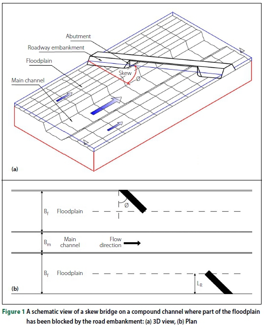
In studying the hydraulics of compound sections, the analysis becomes more complicated when the floodplain experiences a width variation for any reason. Effects of the floodplain cross-section variations will cause the flow to change from uniform to non-uniform and extra momentum/turbulence exchange between the main channel and the floodplain. One reason for this is constructing bridges in compound sections. At the bridge section, some part of the river floodplain is usually blocked for economic reasons (e.g. to reduce span), causing the river to face a contraction in its path during a flood. Figure 1 shows a schematic view of a bridge on a channel with a compound cross-section where the roadway embankment has blocked part of the floodplain with a skew angle 0. In this study, the ratio of the roadway embankment length normal to flow (LR) to the floodplain width (Bf) is defined as the contraction ratio (LR/Bf).
Numerous numerical and experimental studies have been done so far to determine the flow pattern and scouring around rectangular-section bridge abutments. Kandasamy (1989) did extensive studies on the effects of the abutment length on the clear water scouring in a rectangular channel and presented the results for four different zones. Dongol (1994) studied the effects of the abutment length on the scouring and plotted his data with those of Tey (1984) and Kandasamy (1989) for wing-shape abutments, and with those of Kwan (1984) for semicircular abutments, In a similar work, Melville (1997) added more data to those of Dongol (1994) for wing-shape abutments and abutments with vertical and inclined walls.
Molinas et al (1998) performed experiments on vertical abutments for flows with Froude numbers in the range 0.3-0.9 and contraction ratios 0.1, 0.2 and 0.3 (ratio of the abutment length normal to the flow to the total channel width) and showed that the bed shear stress and velocity at the abutment increased up to 10 times compared to those upstream, Ahmed and Rajaratnam (2000) studied the flow field around a wing-shape abutment and concluded that the approaching flow turned into a complex 3D one upstream and around the abutment. They also found that the bed shear stress around the abutment (t/t0) reached a maximum value equal to 3,63 near the nose (t = bed shear stress and t0 = shear stress of the bed approaching flow), Teruzzi et al (2009) studied shear stresses on the bottom wall near the bridge abutment numerically, analysed the 3D flow against the abutment with emphasis on its effects on shear stresses and pressure gradients, and discussed their scouring potentials. Kara et al (2015) studied the effects of the free surface modelling on the flow around the bridge abutments using both the level-set and rigid-lid methods along with the LES (large eddy simulation) turbulence model and showed that the turbulence structure of this flow was strongly influenced by the water surface deformation, while the bed shear stress was quite similar for both models.
Various researchers have studied the flow pattern and scouring around bridge abutments in compound sections besides simple rectangular ones. By proposing a 2D depth-averaged turbulence model for a free surface flow in a 2-stage channel around bridge abutments on the floodplain, Biglari and Sturm (1998) concluded that the measured and computed depth-averaged velocities agreed well, but they emphasised that more 3D studies were needed to check the compound channel effects on the flow characteristics in regions close to obstacles. Sturm and Chrysochoides (1998) experimentally studied scouring around various lengths of bridge abutments under clear water conditions in a compound channel. To predict the scouring depth, Sturm (1999) proposed an equation that depended on local values of hydraulic variables near the nose of the abutment. In another study. Sturm (2006) did some tests on different compound-section geometries considering the main channel-floodplain flow distribution in the contracted section, sediment size, backwater caused by the abutment obstruction, abutment shape, velocity of the approaching flow, and the flow depth. Developing a 2D depth-integrated model and a laboratory hydraulic version, Morales and Ettema (2013) studied the velocity and shear stress in the flow fields around bridge abutments in compound channels, considering different discharges, channel/ abutment geometrical parameters and flow patterns. Using the existing Flow-3D commercial model, Kocaman (2014) evaluated the computational fluid dynamics performance in predicting the water surface level profile at bridges in compound channels with and without piers; the studied bridges were single- and/or double-span with semicircular openings, and single-span with semi-ellipsoid opening. He used the standard k-e turbulence model to estimate the eddy viscosity, compared the numerical and laboratory results, and showed that they conformed well to those of the afflux profile upstream of the bridge. In another study, Atabay et al (2017) proposed an analytical method to calculate the height of afflux around bridges in compound channels. Chua et al (2019) used the LES method to investigate the flow/turbulence structure around varying-length bridge abutments in a channel with an asymmetric compound section.
Another important point in bridge hydraulics is the skew angle and its impact on the flow and bridge-pier scouring, This
has been studied by many researchers so far, e.g. Lança et al (2012), Yang et al (2017), and Shahhosseini and Yu (2019), Studies on the effects of the bridge skew angle on abutments are more limited. Using a 3D numerical model and three groyne angles (45°, 90° and 135°) relative to the upstream flow, Haitigin et al (2007) studied the scouring-hole geometry near the groyne and showed that different lengths/angles of these structures affected it; the highest and lowest erosion belonged to 45° and 135°, respectively, Seckin (2007) performed some tests to study the abutment skew angle effects on the afflux in bridges in compound channels. Using the Flow-3D commercial model, Erduran et al (2012) simulated the flow around bridge skew angles in compound channels and compared the water surface profile with the test results obtained at the Birmingham University Hydraulic Lab; the comparison showed good agreement.
As mentioned earlier, numerical/experimental studies done, so far, to investigate the effects of the contraction ratio on the flow/ scouring pattern in rectangular/compound channels are numerous, but those on the bridge skew angle are few, This study has utilised a 3D numerical model to investigate the simultaneous effects of the bridge skew angle and contraction ratio in compound channels on the flow patterns and the bed shear stress.
Setting up of 3D model
To simulate the flow, the 3D Navier Stokes equations and continuity equation have been used, By considering the Boussinesq approximation with incompressible flow conditions, these will be as follows (Schlichting 1979):
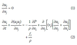
where t, g, P, p, vt,fiand uiare time, gravitational acceleration, pressure, fluid density, eddy viscosity, body force and the velocity Cartesian components in the x¿ directions, respectively. In the present study, the horizontal eddy viscosity (vth) is determined by the Smagorinsky model, while the vertical eddy viscosity (vtv) is computed by the ID k-e model, The horizontal eddy viscosity is specified according to the Smagorinsky model by the following equation (Smagorinsky 1963).
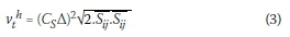
where Csis the Smagorinsky constant varying from 0,1 to 0,8, A is the length scale for the grid filter and Sij is the filtered strain- rate tensor 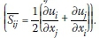
The ID k-e model uses transport equation for turbulent kinetic energy, k, and dissipation of turbulent kinetic energy, e, in the vertical direction, The vertical eddy viscosity from the ID k-e model is as follows:
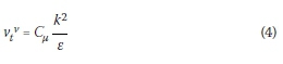
In the above expression, Cuis an empirical coefficient, which is usually a constant equal to 0.09 and k and e are computed from the following transport equations:
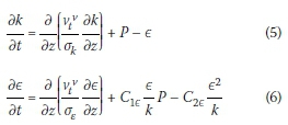
where P =  is the production term due to velocity shear; σk σE, Cle and C2eare empirical parameters with constant values equal to 1, 1.3, 1.44 and 1.92 respectively (MIKE3 2007).
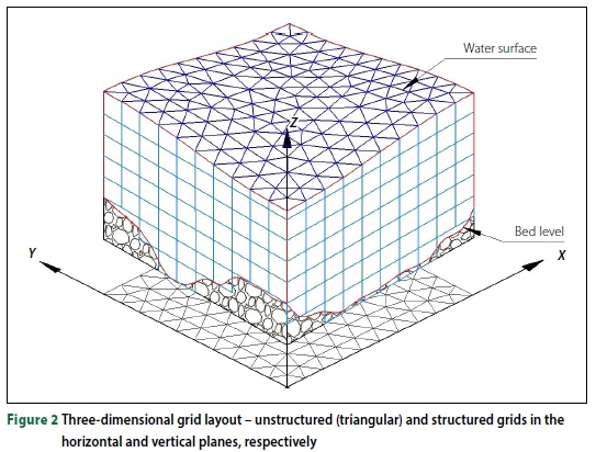
In regions of particular interest, small mesh-size grids will lead to more precise results and the computational domain should have a longer length to either connect the region to the closest known boundary (which may be quite far from the river bridge) or prevent unwanted boundary reflections near the model region; fine grids cause inefficient computations in long regions, One solution to this problem is to use unstructured meshes that form finer grids near the bridge and coarser ones elsewhere in the region; here, an unstructured triangular mesh has been used to discretize the domain in the horizontal direction, and a structured grid has been used to divide it in the vertical direction to form prisms with triangular horizontal faces with similar x and y for each corresponding vertex, Such grids (Figure 2) fit into complicated geometries and enable local mesh refinements.
The finite volume fractional step method was used to solve the governing equations. The transport equation (advection and diffusion) is solved in the horizontal plane using the second-order explicit scheme while the Crank-Nicholson implicit scheme is deployed in the vertical direction. In the developed 3D model, a hydrostatic pressure assumption is applied at top layer cells. More details about boundary conditions, numerical scheme, free surface modelling and solving the system of equations can be found in Namin et al (2004) and Kilanehei et al (2011).
MODEL VALIDATION
To evaluate the performance of the developed numerical model, its results were compared with those of the laboratory tests used on unsymmetrical compound channels to investigate the velocity and shear stress parameters. To assess vortexes, the flow around impermeable groynes were used on one side of the symmetrical compound channel.
Unsymmetrical compound channel
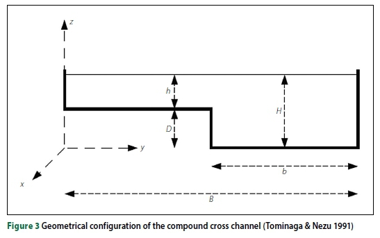
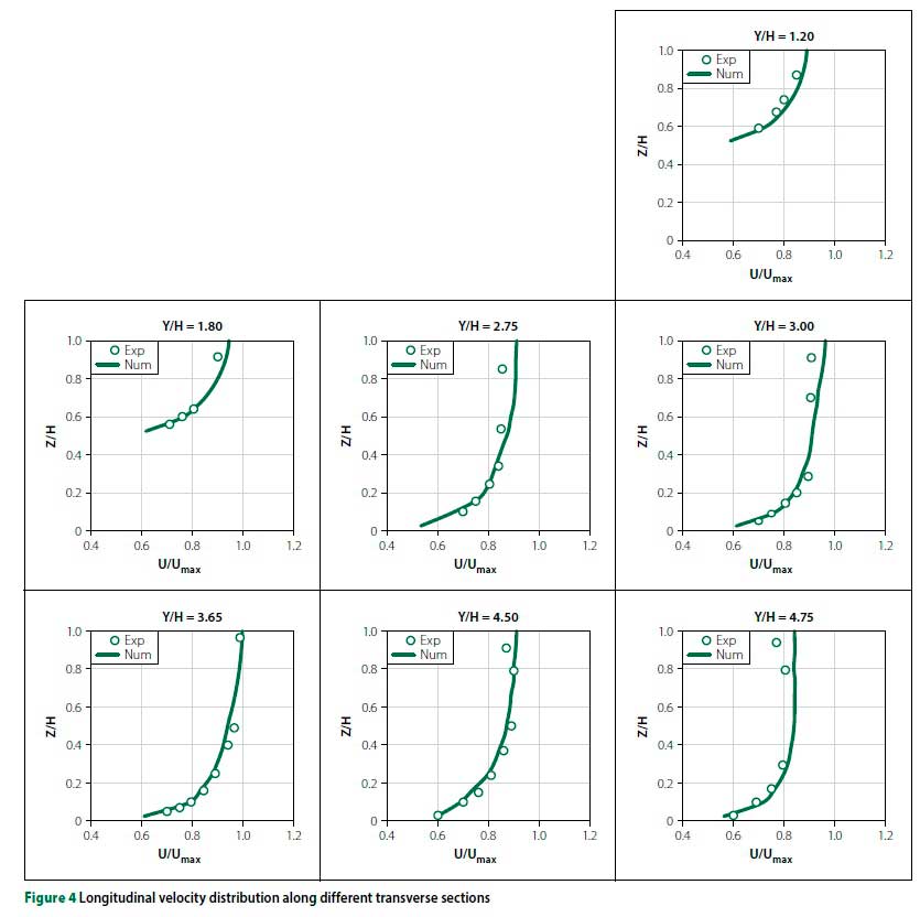
To validate the model for flow simulation capability in compound channels, the laboratory data of Tominaga and Nezu (1991) were used; they did their tests using Laser Doppler Anemometry (LDA). In the laboratory model, the main channel width (b) was 20 cm and the water depth (H) was 8 cm, and there was a floodplain with a width (B-b) equal to 20 cm only on one side (Figure 3). The water depth (h) in the floodplain was 4 cm and the 8 376 cm3/sec discharge was simulated in a flume 12,5 m long with a slope of 0,0006397.
These conditions were also applied to the numerical model. Figure 4 compares the longitudinal velocity distribution along different transverse sections. In this figure, U is the x-direction velocity, Umaxis the maximum x-direction velocity, Y is the y-direction distance from the floodplain wall and Z is the z-direction distance from the main channel bed, The solid-line graph is related to the current numerical study and the dotted one corresponds to the laboratory model, When Y < 20, the section lies in the floodplain and when Y> 20, it lies in the main channel.
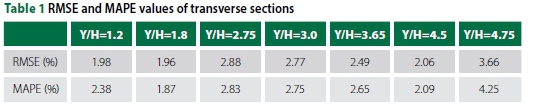
To analyse the results quantitatively, the root mean square error (RMSE) and the mean absolute percentage error (MAPE) were determined as follows:
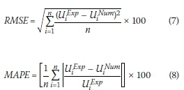
where Num and Exp superscripts represent the numerical and experimental model results, respectively. The RMSE and MAPE values are presented in Table 1 (page 47) for each transverse section. The mentioned values show the accuracy and consistency of numerical prediction. It is worth mentioning that the slight error increase in the numerical calculations at transverse sections near the walls (Y/H = 2.75, Y/H = 3.0 and Y/H = 4.75) could be due to the secondary flows.
As mentioned before, the bed shear stress distribution is important in sediment transport and scouring studies. Bed shear stress distribution for laboratory and current studies are shown in Figure 5; the dots relate to the former and the solid line corresponds to the latter (here twis the average shear stress).
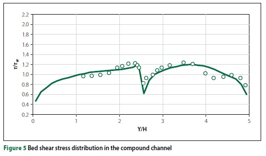
As shown, when the floodplain approaches the main channel junction, the shear stress increases due to their momentum transfer. RMSE and MAE are 9.09% and 7.69%, respectively, showing the accuracy and consistency of the numerical predictions.
Flow around impermeable groynes on one side of the symmetrical compound channel
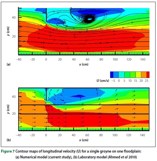
The laboratory data of Ahmed et al (2010) was used to assess the numerical model's flow simulation capability in compound channels with obstacles on its floodplain.
The experiments, conducted at Saitama University in Japan, used a 15 m long, 0.5 m deep, 0.5 m wide symmetrical compound section flume with a main channel width (B) of 0.1 m and a total water depth (H) of 0.24 m, and two symmetrical floodplains with width b equal to 0.2 m (floodplain relative width b/B = 2.0). The flow was a steady type with a discharge (Q) equal to 0.015 m3/s and a floodplain water depth (h) equal to 0.08 m (Figure 6).
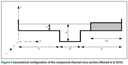
The experiment was conducted using a straight impermeable wooden groyne 0,01 m thick and a relative length (groyne length L to the floodplain width) of 0,75 fixed vertically to the main channel centerline and to the flow direction (Ahmed et al 2010).
Similar conditions were applied to the developed model for which the contour maps of the longitudinal velocity (U) are shown in Figure 7 where vortices are formed at the groyne downstream, The flow is totally one-way in the laboratory and proposed numerical models at distances 6.67 and 7.46 times the groyne length, respectively, and the maximum vortex width occurs in them at 1.65 and 1.6 times the groyne length, respectively, concluding that the numerical predictions are accurate and consistent.
Results
To perform the current study, some dimensions were assumed for the symmetrical compound channel's cross-section. Floodplain width (Bj) is 140 m, main channel width (Bm) is 70 m, the height difference between the main channel bottom and the floodplain beds is 2 m, the height difference between the floodplain beds and the roadway surface is 5 m, the slope of the sidewalls of the main channel and floodplains is 45 degrees, and the channel's longitudinal slope is 0.0005 (Figure 8 on page 49). The roughness of the main channel bed differs from that of the floodplain; hence, it has been taken as 0.03 for the main channel and 0.05 for the floodplain in all the related simulations. The bridge abutment width in the roadway is 11 m and the slope of the route's side embankments is 3 (horizontal) to 1 (vertical), Also, LRis the vertical projection of the roadway embankment.
The effects of the roadway contraction ratio (LR/Bf) and skew angle (0) on the velocity distribution and bed shear stress have been studied in this research, where the flow-splitting and flow-guiding embankments are expressed, for simplicity, as northern and southern abutments, respectively.
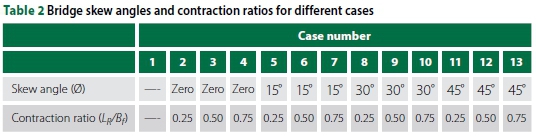
Thirteen cases, with bridge skew angles and contraction ratios as shown in Table 2 (page 49), were considered to study the issue with the numerical model (Case 1 had no bridges) based on the variables shown in Figure 8.
Velocity distribution at the bridge location
Figures 9-11 show the velocity values and streamlines in plan for Cases 2-13 (items for each contraction ratio are shown separately).
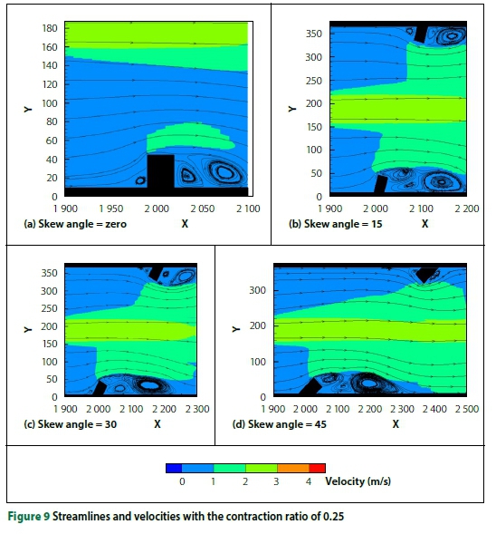
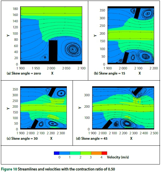
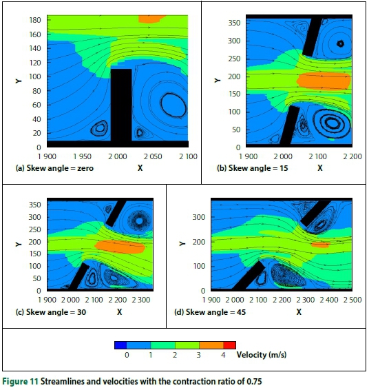
These figures show how the flow and velocity are distributed across the bridge. Horizontal vortices, formed mainly behind the abutments, are also visible.
The dimensionless ratio of the maximum velocity in the main channel is shown in Figure 12 where Vmax0 is the maximum velocity in the main channel (Case 1 in Table 2, no-bridge compound channel), Vmax-mcis the maximum velocity in the main channel area and CR is the contraction ratio.
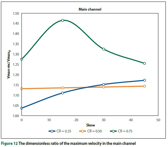
As shown, when the contraction ratio equals 0.25, an increased skew angle increases the maximum velocity so that at a 45° skew angle (Case 11) the increase is 15% compared to the zero skew angle mode (Case 2). A point worth noting is that, in the main channel, the maximum velocity does not necessarily occur exactly along the bridge axis (parallel to the route); it may increase slightly before or after the bridge location where the southern abutment skew angle seems to direct the flow in the entire opening width along the bridge axis, which reduces the velocity exactly at the bridge location. A more uniform discharge distribution along the bridge direction reduces the peak velocity in the bridge opening.
When the contraction ratio equals 0.50, an increased skew angle does not change the maximum velocity considerably, because the flows forming behind and in front of the northern and southern abutments do not change significantly, resulting in a more uniform discharge distribution. In this case, the maximum velocity occurs along the bridge axis, except at a skew angle of 45° where it occurs slightly before and after the bridge.
Conditions change somewhat when the contraction ratio equals 0.75. In the main channel with a 15° skew angle, the velocity is 20% more than that with a 0° skew angle, and when the skew angle tends to 45°, the maximum velocity in the main channel nearly equals the no-skew angle mode. In this case, by increasing the skew angle from 15° to 30° and 45°, the length of the road embankment is increased and necessary space is provided to create a recirculation zone upstream of the northern abutment. The formation of this zone guides the flow to the main channel and reduces the peak velocity.
Figure 13 shows the dimensionless ratio of the maximum velocity around the southern abutment (Vmax-sa) in a bridge-affected area for different contraction ratios. As shown, at all skew angles the maximum velocity around this abutment increases with an increase in the contraction ratio, and the maximum increase (for a fixed skew angle) is related to a 15° skew angle where the difference between contraction ratios of 0.25 and 0.75 is about 164%. The figure also shows that, at all three contraction ratios, an increase in the bridge skew angle reduces the maximum velocity around the southern abutment. The maximum velocity reduction rates at contraction ratios of 0.25, 0.50 and 0.75 are 21%, 46% and 36%, respectively.
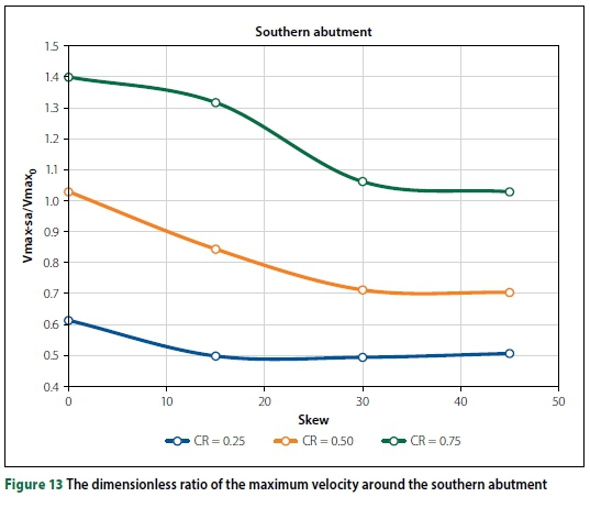
According to the flow pattern formed upstream of the southern abutment, it can be concluded that the skew angle causes the southern abutment to act as a guide wall leading the flow uniformly into the main channel at the bridge location which reduces the flow-abutment confrontation.
Around the northern abutment, the situation is more complicated, and Figure 14 shows the dimensionless ratio of the maximum velocity around this abutment (Vmax_na) for different contraction ratios.
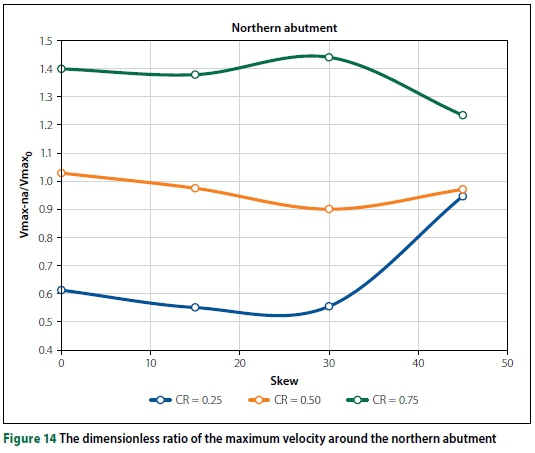
As shown, the general trend at contraction ratios of 0.25 and 0.50 is similar for different skew angles; with an increase in the skew angle up to 30°, the maximum velocity around the northern abutment has slightly reduced, but at a skew angle of 45°, it has increased again (more so for a contraction ratio of 0.25), For skew angles < 30°, the channel's extended width (along the bridge length) allows the flow to adapt itself to the abutment shape and pass the bridge opening almost evenly, but at a skew angle of 45° the flow-abutment confrontation increases so much that the velocity around the northern abutment is increased. At a contraction ratio of 0.75 where the flood passage gets narrower and the skew angle increases up to 30°, the flow-abutment confrontation causes the maximum velocity to increase slightly around the northern abutment, but at a skew angle of 45° the dead zone formed upstream of this abutment widens and adjusts the flow circulation so that it passes the bridge opening almost uniformly, causing the maximum velocity to reduce around this abutment.
As mentioned before, the flow around the northern abutment is more complex than that around the southern one because there is a flow-abutment confrontation. Conditions are so complex that defining a specific trend for the flow passing the bridge is very difficult, because the channel and bridge geometry are quite influential, and each case needs careful study. However, as was predicted, at a skew angle of 0, the increase in the contraction ratio (the decrease in the bridge span) causes the velocity to increase considerably around the northern and southern bridge abutments, The velocity increased by 67% when the contraction ratio increased from 0.25 to 0.50 and by 40% when it increased from 0.50 to 0.75. This velocity increase around the northern abutment can also be observed for the contraction ratio increase for other skew angles (15°, 30° and 45°), with the only difference being at a skew angle of 45° where the percent velocity increase is lower than those of the other cases due to the formation of a dead zone behind the northern abutment.
Another interesting point is that the maximum velocity in the main channel, around the northern abutment and southern abutment, occurs at a contraction ratio of 0,75 and skew angles of 15°, 0° and 30°, respectively, Maximum velocity values are almost equal to each other.
Shear stress at the bridge location
The shear stress parameter is another important flow hydraulic criterion at the bridge abutment, Figure 15 (where Smax0 is the maximum shear stress in the whole section in the no-roadway embankment mode) shows the nondimensionalised maximum shear stress around the southern abutment (Smax-sa) for different contraction ratios.
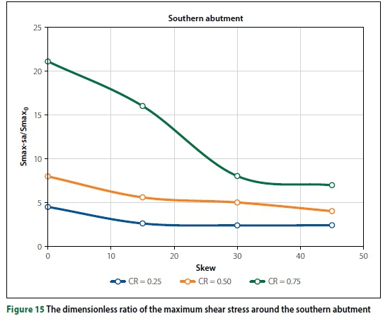
As shown, for all contraction ratios an increased skew angle reduces the maximum shear stress around the southern abutment. This reduction is moderate at contraction ratios of 0.25 and 0.50, and severe at a contraction ratio of 0.75 (especially at skew angles 0°-30°), For a constant skew angle, as the contraction ratio increases, the maximum shear stress increases, and results confirm this.
As mentioned earlier, conditions were more complex around the northern abutment, Figure 16 shows the dimensionless ratio of the maximum shear stress around the northern abutment (Smax_na) for different contraction ratios, When it is 0.25, the maximum shear stress does not change much for skew angles up to 30°, but at a skew angle of 45° the shear stress almost doubles in the northern abutment zone due to the flow-abutment confrontation.
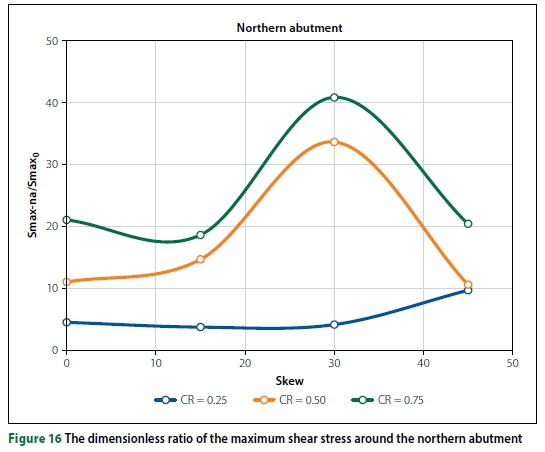
At contraction ratios of 0,50 and 0,75, the maximum shear stress is higher than the 0.25 case, but with a different trend, In these contraction ratios, changes are small at skew angles of zero and 15°, but at 30° the stress is increased considerably due to the flow-abutment confrontation, In both 0.50 and 0.75 contraction ratios, the maximum shear stress decreases sharply due to an increase in the skew angle up to 45° and reaches to about the zero-skew angle case. This is also due to the formation of a dead zone upstream of the abutment that acts like a guide wall causing a uniform flow and a reduction in the maximum shear stress around the northern abutment.
CONCLUSIONS
Determining the flow field and bed shear stress is a necessity for studying the scour of bridges, Since the bridge skew angle and the contraction ratio are the factors that affect the hydraulic performance of river bridges, this paper has studied the flow around bridges in compound channels with different contraction ratios (0.25, 0.50 and 0.75) and various skew angles (0°, 15°, 30° and 45°), Accordingly, a 3D flow model was developed and utilised after its validation by various cases.
When a bridge has a skew angle, one of the abutments directs the flow throughout the opening width, reduces the flow velocity along the bridge axis, and decreases the maximum velocity in the bridge opening due to a more uniform discharge distribution in this direction, especially at small contraction ratios.
When both the bridge skew angle and the contraction ratio are high, the maximum velocity occurs along the bridge axis, instead of in the main channel around the northern abutment where, in general, the flow velocity pattern is complex and determining a similar process for different states is difficult. On the other hand, the maximum velocity around the northern abutment increases for every skew angle, with an increase in the contraction ratio. Again, an increase in the bridge skew angle reduces the maximum velocity around the southern abutment, because the skew angle will cause the roadway embankment to act as a guide wall leading to a uniform flow towards the main channel at the bridge location.
With regard to the bed shear stress, when the contraction ratio does not vary, an increase in the bridge skew angle reduces the maximum shear stress around the southern abutment, and this decrease is more at larger contraction ratios. An increased contraction ratio increases the maximum shear stress around the mentioned abutments.
Shear stress conditions are also complicated around the northern abutment; at low contraction ratios, the maximum shear stress does not change much at bridge skew angles of up to 30°, but at 45° the shear stress almost doubles in the northern abutment region due to the flow-abutment confrontation. A point worth noting here is the decrease in the maximum shear stress with an increase in the bridge skew angle when the contraction ratio is high. This, too, can be due to the formation of an upstream flow dead zone that acts like a guide wall causing a uniform flow passage that decreases the maximum shear stress around the northern abutment.
REFERENCES
Ahmed, F & Rajaratnam N 2000. Observations on flow around an abutment. Journal of Engineering Mechanics, 125(1): 51-59. [ Links ]
Ahmed, H S, Hasan, M M &Tanaka, N 2010. Analysis of flow around impermeable groynes on one side of symmetrical compound channel: An experimental study. Water Science and Engineering, 3(1): 56-66. [ Links ]
Aksoy, A O & Eski, O Y 2016. Experimental investigation of local scour around circular bridge piers under steady state flow conditions. Journal of the South African Institution of Civil Engineering, 58(3): 21-27. [ Links ]
Atabay, S, Haji Amou Assar, K, Hashemi, K & Dib, M 2017. Prediction of the backwater level due to bridge constriction in waterways. Water and Environment Journal, 32(1): 1-10. [ Links ]
Biglari, B & Sturm, T W 1998. Numerical modeling of flow around bridge abutments in compound channel. Journal of Hydraulic Engineering, 124(2): 156-164. [ Links ]
Chua, K V, Fraga, B, Stoesser, T, Hong, S H & Sturm, T 2019. Effect of bridge abutment length on turbulence structure and flow through the opening. Journal of Hydraulic Engineering. 145(6): 04019024. [ Links ]
Dongol, D M S 1994. Local scour at bridge abutments. Report No. 544. Auckland, New Zealand: University of Auckland, School of Engineering. [ Links ]
Erduran, K S, Seckin, G, Kocaman, S & Atabay, S 2012. 3D Numerical modeling of flow around skewed bridge crossing. Engineering Applications of Computational Fluid Mechanics, 6(3): 475-489. [ Links ]
Haitigin, W, Biron P & Lapointe M 2007. Predicting equilibrium scour-hole geometry near angled stream deflectors using a three-dimensional numerical flow model. Journal of Hydraulic Engineering, 133(8): 983-988. [ Links ]
Kandasamy, J K 1989. Abutment scour. Report No. 458. Auckland, New Zealand: University of Auckland, School of Engineering. [ Links ]
Kara, S, Kara, M C, Stoesser, T & Sturm, T W 2015. Free-surface versus rigid-lid LES computations for bridge-abutment flow. Journal of Hydraulic Engineering, 141(9): 04015019. [ Links ]
Kilanehei, F, Naeeni S T O & Namin M M 2011. Coupling of 2DH-3D hydrodynamic numerical models for simulating flow around river hydraulic structures. World Applied Sciences Journal, 15(1): 63- 77. [ Links ]
Kocaman, S 2014. Prediction of backwater profiles due to bridges in a compound channel using CFD. Advances in Mechanical Engineering, 6: 905217. [ Links ]
Kwan, F 1984. Study of abutment scour. Report No. 328 Auckland, New Zealand: University of Auckland, School of Engineering. [ Links ]
Lança, R, Fael, C, Maia, R, Pego, J & Cardoso, A H 2012. Effect of spacing and skew-angle on clear-water scour at pier alignments. Proceedings, International Conference on Fluvial Hydraulics (River Flow 2012), 5-7 September 2012, San José, Costa Rica, pp 927-933. [ Links ]
Melville, BW 1997. Pier and abutment scour: Integratec approach. Journal of Hydraulic Engineering, 123(2): 125-136. [ Links ]
MIKE 3 2007. Hydrodynamic module. Scientific Documentation, DHI software. http://www.mikepoweredbydhi.com. [ Links ]
Molinas, A, Kheireldin, K & Wu, B 1998. Shear stress around vertical wall abutments. Journal of Hydraulic Engineering, 124(8): 822-830. [ Links ]
Morales, R & Ettema, R 2013. Insights from depth-averaged numerical simulation of flow at bridge abutments in compound channels. Journal of Hydraulic Engineering, 139(5): 470-481. [ Links ]
Namin M M, Lin, B & Falconer, R A 2004. Modeling estuarine and coastal flows using an unstructured triangular finite volume algorithm. Journal of Advances in Water Resources, 27(12): 1179-1197. [ Links ]
Schlichting, H 1979. Boundary Layer Theory. New York: McGraw-Hill. [ Links ]
Seckin, G 2007. The effect of skewness on bridge backwater prediction. Canadian Journal of Civil Engineering, 34(10): 1371-1374. [ Links ]
Shahhosseini, M & Yu, G 2019. Experimental study on the effects of pier shape and skew angle on pier scour. Proceedings, 3rd International Conference on Fluid Mechanics and Industrial Applications, 29-30 June 2019, Taiyun, China. Journal of Physics Conference Series, Vol 1300. DOI; 10.1088/1742-6596/1300/1/012031. [ Links ]
Smagorinsky. J 1963. General circulation experiment with the primitive equations. Monthly Weather Review, 91: 99-165. [ Links ]
Sturm, T W & Chrisochoides, A 1998. Abutment scour in compound channels for variable setbacks. Proceedings, ASCE International Water Resources Engineering Conference, Memphis, TN, pp 174-179. [ Links ]
Sturm, T W 1999. Abutment scour in compound channels. In Stream Stability and Scour at Highway Bridges. Compendium of Papers - ASCE Water Resources, Reston, VA, pp 443-456. [ Links ]
Sturm, T W 2006. Scour around bankline and setback abutments in compound channels. Journal of Hydraulic Engineering. 132(1): 21-32. [ Links ]
Teruzzi, A, Ballio, F & Armenio, V 2009. Turbulent stresses at the bottom surface near an abutment; Laboratory-scale numerical experiment. Journal of Hydraulic Engineering, 135(2): 106-117. [ Links ]
Tey, C B 1984. Local scour at bridge abutments. Report No. 329. Auckland, New Zealand: University of Auckland, School of Engineering. [ Links ]
Tominaga, A & Nezu, 11991. Turbulent structure in compound open-channel flows. Journal of Hydraulic Engineering, 117(1): 21-41. [ Links ]
Yang, Y, Melville, B W, Shamseldin, A Y & Friedrich, H 2017. Effect of skewness on clear-water local scour at complex bridge piers. Proceedings, 37th International Association for Hydro-Environment Engineering and Research (IAHR) World Congress, 13-18 August 2017, Kuala Lumpur, Malaysia, pp 13-18. [ Links ]
 Correspondence:
Dr Amir Mahjoob
Transportation Research Institute, Housing and Urban Development Research Centre
Tehran, Iran
T: +98 912 547 6651
E: a.mahjoob@bhrc.ac.ir
Dr Fouad Kilanehei
Assistant Professor
Department of Civil Engineering, Imam Khomeini International University
Qazvin, Iran
T: +98 912 281 5532
E: kilanehei@eng.ikiu.ac.ir

DR AMIR MAHJOOB, who has 16 years' academic and research experience in the field of hydraulic structures engineering, received his PhD degree from the University of Tehran, Iran. He has been working at the Road, Housing and Urban Development Research Centre as an Assistant Professor since 2014. His research interests are in bridge hydraulics, river engineering, numerical simulation of flow and sediment, and flood hazards. Currently he directs several research projects regarding hydraulic inspection of river bridges, bridge scour and stream instability countermeasures.

DR FOUAD KILANEHEI is an Assistant Professor in the Civil Engineering Department at Imam Khomeini International University, Iran. He worked in the river bridge design control division of the Ministry of Roads and Transportation of Iran for eight years before joining the Imam Khomeini International University in 2013 as scientific member. He received his PhD and MSc degrees in Hydraulic Structures from the University of Tehran, Iran. His current and main research interests are physical modelling and development of numerical models.

