TECHNICAL PAPER

 

Estimation of areal reduction factors using daily rainfall data and a geographically centred approach

 

 

OJ Gericke; J P J Pietersen

Correspondence

 

 

---

ABSTRACT

This paper presents the estimation of geographically centred and probabilistically correct areal reduction factors (ARFs) from daily rainfall data to explain the unique relationship between average design point rainfall and average areal design rainfall estimates at a catchment level in the C5 secondary drainage region in South Africa as a pilot case study. The methodology adopted is based on a modified version of Bell's geographically centred approach. The sample ARF values estimated varied with catchment area, storm duration and return period, hence confirming the probabilistic nature. The derived algorithms also provided improved probabilistic ARF estimates in comparison to the geographically and storm-centred methods currently used in South Africa. At a national level, it is envisaged that the implementation and expansion of the methodology will ultimately contribute towards improved ARF estimations at a catchment level in South Africa. Consequently, the improved ARF estimations will also result in improved design flood estimations.

Keywords: areal rainfall, areal reduction factor, design rainfall, geographically centred, point rainfall, probabilistic, design flood estimation

---

 

 

INTRODUCTION

In general, observed rainfall data can be obtained from continuously recording rainfall stations or from daily rainfall stations. In South Africa, daily rainfall data is recorded at a fixed daily interval and is more abundant, reliable and generally have longer record lengths than the digitised sub-daily rainfall data (Smithers & Schulze 2000b; 2004). Hence, due to the availability and quality of daily rainfall data, these data sets are more often used to estimate design rainfall. Design rainfall is derived from observed rainfall data and comprises a depth and duration associated with a given return period (T) or annual exceedance probability (AEP) (Gericke & Du Plessis 2011), Design rainfall for durations < 24-h is normally classified as 'short duration design rainfall and is generally estimated directly from continuously recorded rainfall. 'Long duration' design rainfall typically ranges between one and seven days and can be estimated from both continuously recorded and daily rainfall data, However, design point rainfall estimates are only applicable to a limited area, and for larger areas, the average areal design rainfall depth is likely to be less than the maximum design point rainfall depths (Siriwardena & Weinmann 1996), Areal reduction factors (ARFs) are used to describe this relationship between design point and areal design rainfall, i.e. design point rainfall depths are converted to an average areal design rainfall depth for a catchment-specific critical storm duration and catchment area (Alexander 2001).

Numerous factors can have a significant impact on the estimation of ARFs, e.g. geographical location, rainfall types, catchment geomorphology, and methodological approaches (Asquith & Famiglietti 2000; Svensson & Jones 2010; Li et al 2015). In terms of geographical location, it has been shown that the 1-day ARFs in the United States of America (USA) exceeded the equivalent ARF estimates in Australia, while the ARFs decline more rapidly in the semi-arid southwestern USA than in the rest of the USA (Svensson & Jones 2010), Different rainfall-producing mechanisms, e.g. convective versus frontal rainfall, will produce different spatial rainfall patterns and consequently result in different ARF values (Eggert et al 2015). For example, Skaugen (1997) established that ARFs for both convective and frontal rainfall decrease with increasing return period, but the rate of decrease for convective rainfall is noticeably larger than that for frontal rainfall. In the USA, areal rainfall was found to decrease in comparison with the corresponding point rainfall with increasing return periods (Asquith & Famiglietti 2000; Allen & DeGaetano 2005), In contrast, Grebner and Roesch (1997) demonstrated that ARFs in Switzerland (catchment areas > 4 500 km²) are independent of the return period, Most studies conducted on the estimation of ARFs have concluded that catchment geomorphology (e,g, area, shape and topography) and topographical rainfall biases (e,g, leeward and windward effects) have an insignificant influence on ARFs (Allen & DeGaetano 2005; Svensson & Jones 2010), However, Singh et al (2018) highlighted that differences in ARFs in New Zealand are ascribed to differences in topography and rainfall type, Kim et al (2019) also showed that storm-centred ARF values obtained from storms of a different shape, i,e, elliptical versus circular, could be different by up to 20%, In catchment areas less than 800 km², ARFs are generally a function of the point and areal rainfall intensity, as the relationship between rainfall intensity and soil infiltration is pre-dominant, In catchment areas greater than 800 km² and less than 30 000 km², ARFs are mainly a function of the area and storm duration (Alexander 2001; SANRAL 2013).

ARFs can be estimated using either analytical or empirical methods (Pietersen et al 2015), The first analytical methods were based on simplified algorithms and limited verification processes (Siriwardena & Weinmann 1996; Svensson & Jones 2010), Hence, several new analytical methods have been proposed during the last four decades, e,g, storm movement (Bengtsson & Niemczynowicz 1986), crossing properties (Bacchi & Ranzi 1996), spatial correlation structure (Sivapalan & Blöschl 1998), scaling relationships (De Michéle et al 2001), and temporal-spatial rainfall dependence (Mineo et al 2018), Empirical methods could be classified as either geographically centred or storm-centred approaches, The geographically centred approach describes the relationship between average areal design rainfall over a geographically fixed area and a corresponding design point rainfall value, In the storm-centred approach, the estimation of average areal design rainfall is not limited to a fixed geographical area, but rather associated with the extent of individual dynamic storm rainfall events and the way in which the rainfall intensity decreases with distance from the central maximum rainfall core (Alexander 2001; Svensson & Jones 2010).

Internationally, extensive national-scale ARF studies are limited to the United Kingdom (NERC 1975), USA (USWB 1957; 1958) and Australia (Siriwardena & Weinmann 1996; Podger et al 2015), Due to insufficient rainfall monitoring networks and a lack of short duration rainfall data, most of the data-intensive analytical and empirical methods developed often fail to successfully incorporate the variation in predominant weather types, storm durations, seasonal factors and return periods (Skaugen 1997; Asquith & Famiglietti 2000; Allen & DeGaetano 2005, Pavlovic et al 2016), In recent years, radar information has also become more readily available in many parts of the world and assists in improving the spatial and temporal resolutions to estimate ARFs, e,g, Peleg et al (2018) and Kim et al (2019). According to Pavlovic et al (2016), the differences between analytical and empirical ARF estimation methods currently in use are also more pronounced for shorter storm durations and larger catchment areas, while being partially dependent on the return period, Thus, in general, most of these methods are inappropriate to use at a comprehensive set of temporal and spatial scales in larger catchments, Similarly, in South Africa the estimation of ARFs is limited to the storm-centred approaches of Van Wyk (1965) and Wiederhold (1969), while Alexander (2001) also developed a geographically centred approach based on the UK Flood Study Report (FSR) methodology.

The Van Wyk (1965) study was conducted on a small scale (catchment areas < 800 km²) in the Pretoria region, Gauteng, to derive probabilistically correct ARF values which vary with return period, Wiederhold (1969) used a modified version of the Van Wyk (1965) method to establish ARFs for 170 storms over large catchment areas between 500 km² and 30 000 km² within 18 regions delineated for South Africa. However, the latter ARFs are regarded as being probabilistically incorrect, since the ARF estimates remain constant irrespective of the return period under consideration, In the case of Alexander (2001), the UK FSR methodology was adjusted to account for short duration rainfall over small catchment areas, since it was argued that estimates of shorter duration rainfall based on the extrapolation from longer durations are unreliable when viewed in the light of the storm mechanisms which produce high-intensity rainfall for durations less than ten minutes, Hence, with the latter adjustments being implemented, the practitioner can estimate average catchment rainfall from point rainfall statistics using a geographically centred approach, However, as in the case of Wiederhold (1969), the ARF values are also regarded as probabilistically incorrect, Nowadays, the local derivation of probabilistically correct ARFs is also regarded as problematic due to the overall deterioration of our rainfall monitoring network, both in terms of data availability, quality and resolution.

Based on the shortcomings highlighted above, it is clear that the estimation of ARFs is internationally an on-going research question, particularly in South Africa. Typically, practitioners would use storm-centred derived ARFs in a geographically centred sense, which will most probably then result in either an over- or underestimation of the actual fixed-area storm event, Hence, the primary objective of this study is to estimate geographically centred ARFs using daily rainfall data and a modified version of Bell's method (1976) to derive the unique relationship between average design point rainfall and average areal design rainfall estimates at a catchment level, Consequently, this will investigate how ARF values vary with catchment area (400 km²<A< 5 000 km²), rainfall type and storm duration (1, 8, 16, 24, 72 and 168 hours), and return period (2 - 200 years) in 23 quaternary catchments of the C5 secondary drainage region in South Africa, The specific objectives are to:

■ establish mathematical relationships between the estimated ARFs and rainfall variables (e,g, mean annual precipitation (MAP), storm duration and return period), catchment geomorphology (e,g, area, shape and geographical location), and/or a combination of these, and

■ compare the derived ARF algorithms with a selection of empirical ARF methods currently used in South Africa in order to assess any differences

 

MATERIALS AND METHODS

This section provides a general overview of the study area and the detailed methodology applied.

Study area

The pilot study area (C5 secondary drainage region), as shown in Figure 1, covers 34 795 km² and is situated within the larger primary drainage region C in South Africa (DWAF 1995), The C5 secondary drainage region is one of 148 secondary drainage regions found in South Africa and is further divided into two tertiary drainage regions, namely the Riet River (C51) and Modder River (C52) catchments, which are further subdivided into 23 quaternary catchments, e.g. C51A, C51B to C52L (Midgley et al 1994).

 

 

The pilot study area is located in a summer rainfall region characterised by convective rainfall. The average MAP is 424 mm and decreases from 685 mm in the east to 275 mm in the west (Lynch 2004), The rainy season starts in early September and ends in mid-April with a dry winter following, The topography is gentle with elevations varying from 1 021 m to 2 120 m above mean sea level. The average catchment slopes vary between 1,7% and 10,3% (USGS 2016). The 223 South African Weather Services (SAWS) daily rainfall stations located within and close to the boundary of the pilot study area are shown in Figure 2. It is evident from Figure 2 that the daily rainfall monitoring network is generally denser in the mid-eastern parts of the pilot study area as opposed to the northwestern parts. The minimum number of rainfall stations in each of the 23 quaternary catchments (C51A - C52L) is based on the criteria recommended by Siriwardena and Weinmann (1996), i.e. a minimum of three rainfall stations for catchment areas up to 500 km² plus one additional station for every 500 km² thereafter.

 

 

Extraction, infilling and averaging of observed point and areal rainfall

A daily rainfall database was established by evaluating, preparing and extracting daily rainfall data from the SAWS rainfall stations present in the pilot study area, as well as from the neighbouring rainfall stations. The Daily Rainfall Extraction Utility (DREU) (Lynch 2004) was used for the extraction of the daily rainfall data series, In considering the impact that an incomplete month and consequently an incomplete year could have on the record length of a particular rainfall station, the default infilling techniques available in the DREU, e.g. inverse distance weighting, expectation maximisation, median ratio and/or monthly infilling, were used for the infilling of missing daily rainfall data, Infilling of daily rainfall values was necessary in some cases to obtain a minimum record length of at least 30 years.

The 1-day fixed time interval point rainfall annual maximum series (AMS) was firstly identified and extracted from the observed rainfall data, In order to obtain the 3-day and 7-day fixed time interval point rainfall AMS, a 'moving window' approach was applied to the 1-day fixed time interval point rainfall to provide the accumulated 3-day and 7-day totals, respectively, The highest accumulated values within each hydrological year were then used as the 3-day or 7-day fixed time interval point rainfall AMS values. This process was repeated for each hydrological year to result in a complete 3-day and 7-day fixed time interval point rainfall AMS at each rainfall station. The 1-day, 3-day and 7-day point rainfall AMS at each rainfall station were then multiplied with corresponding Thiessen weights to provide a single, weighted point rainfall AMS representative of all the rainfall stations within a particular quaternary catchment, The use of the Thiessen polygon method (Wilson 1990) is justified by the even spatial distribution of the rainfall stations and the relatively flat topography of the pilot study area, while it was also the preferred method in various international ARF studies, e.g. Bell (1976), Stewart (1989), Siriwardena and Weinmann (1996), and Podger et al (2015), In considering the large amount of data and repetitive computations required, using the Create Thiessen Polygons extension in the ArcGIS™ environment further simplified the process and ensured that a consistent approach was followed.

In terms of obtaining the areal rainfall AMS, the same procedure was followed, except for the Thiessen weighting procedure, In the latter case, catchment rainfall values were determined by multiplying the daily rainfall values with a corresponding Thiessen weight to result in a weighted daily catchment rainfall series, Thereafter, the areal AMS values were extracted from the estimated daily catchment rainfall series.

Disaggregation of fixed interval rainfall

The fixed time interval point and areal rainfall AMS at each rainfall station were disaggregated to continuous measures of K-hour rainfall using the methodology as proposed by Smithers and Schulze (2003; 2004) and as subsequently implemented in the C5 secondary drainage region by Gericke and Pietersen (2018), In essence, for storm durations exceeding 24-h, the K-day fixed time interval point and areal AMS values were converted to continuous measures of K-hour rainfall using the conversion factors proposed by Adamson (1981) for selected storm durations, e,g, 1,11 for 1-day to 24 hours, 1,05 for 3-days to 72 hours, and 1,02 for 7-days to 168 hours, For storm durations < 24-h, the scaling factors proposed by Smithers and Schulze (2003) were used to downscale the mean of the 24-h AMS values to ultimately obtain the K-hour (e.g. 1-h, 8-h, 16-h and 24-h) point and areal AMS values.

Probabilistic analysis of point and areal rainfall

The selection of the most suitable theoretical probability distribution was based on the statistical properties (mean, standard deviation, skewness and coefficient of variation) of each point and/or areal rainfall AMS, Typically, the Log Normal (LN), Log-Pearson Type 3 (LP3), General Extreme Value (GEV) and Generalised Logistic (GLO) probability distributions were considered for the frequency analyses, and the probable weighted moments (PWM) and linear moments (LM) were used to estimate parameters for the purpose of probabilistic curve fitting, However, Smithers and Schulze (2000a) highlighted that the GEV probability distribution is regarded as the most suitable distribution to estimate 1-day design rainfall values in South Africa, while the GEV probability distribution was also used to estimate ARFs in various other international studies, e,g, Dyrrdal et al (2016) and Peleg et al (2018), Therefore, based on the aforementioned recommendations, the GEV distribution was utilised in this study for the probabilistic curve fitting, The probabilistic analyses of the point and areal rainfall AMS were conducted separately to result in separate design point and areal design rainfall frequency curves, In essence, the design point rainfall values were firstly estimated from a single set of Thiessen-weighted AMS values as obtained from multiple rainfall stations in each catchment, This approach was used to provide a catchment-based design point rainfall frequency curve, The following steps were followed:

a. Extraction of the point rainfall AMS values at each rainfall station within a particular quaternary catchment.

b. Weighting of the point rainfall AMS values using Thiessen polygons to result in weighted point rainfall AMS values representative of all the rainfall stations in a particular quaternary catchment.

c. Estimation of the first four PWMs (ß₁ ß₂, ß₃and ß₄) and subsequent four L-Moments (λ₁ λ₂, λ₃ and λ₄) having at least 30 years of data (> 60 years preferred).

d. Estimation of the shape parameter (k in Equation 1), coefficient of the shape parameter (c in Equation 2), location parameter (e in Equation 3) and scale parameter (a in Equation 4) as required for the GEV distribution:

where t₃is L-skewness of the data set, T is the gamma function and λ₁and λ₂ are the first and second L-moments, respectively.

e. Estimation of the regional T-year design point rainfall value P_ps(T)in Equation 5) and associated AEP (Equation 6) by fitting the parameters to the GEV distribution:

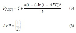
Similarly, probabilistic analyses of the areal rainfall AMS (extracted and weighted at a daily time interval) were conducted at a quaternary catchment level to result in a single representative areal frequency curve which condenses information from all the areal rainfall AMS within a particular quaternary catchment, As mentioned before, the areal AMS values were estimated by multiplying a representative Thiessen weight, at a daily time interval, with the corresponding daily rainfall values, This procedure resulted in one areal AMS applicable to a particular quaternary catchment. Subsequently, a similar probabilistic curve-fitting procedure as listed above was applied to the areal AMS to result in a single set of T-year areal design rainfall values (P_as(t)) applicable to each quaternary catchment under consideration.

Estimation of areal reduction factors

The estimation of ARFs is based on a 'modified version' of Bell's (1976) method, since the AMS of point and areal rainfall are used as opposed to the partial duration series (PDS) used by Bell (1976), This adjustment from the PDS to the AMS will incorporate the variation of ARFs with AEPs, instead of possibly excluding the highest observed rainfall value in a specific hydrological year by using equally ranked observations from a common base period. The ARFs were expressed as the ratio of areal to average design point rainfall with associated AEPs. Sample values of the fixed-area ARFs were estimated using steps (a) to (e) as described in the previous section and expressed using Equation 7, i,e, the ratio between the catchment areal design rainfall and the average design point rainfall estimates for corresponding return periods.

where ARF_Tis the areal reduction factor at a specific return period (%), -P_AS(T) is the catchment T-year areal design rainfall (mm), and P_PS(T) is the average T-year design point rainfall (mm).

One set of ARFs was estimated for each quaternary catchment with storm durations of 1, 8, 16, 24, 72 and 168 hours with corresponding return periods of 2, 5, 10, 20, 50, 100 and 200 years, The ARFs from individual quaternary catchments were pooled together to estimate sample ARFs for a combination of catchment areas, storm durations, MAP and T values at a tertiary catchment level, These sample ARF values were then used to derive functional ARF algorithms, which are discussed in the next section.

Derivation of regressions to estimate ARFs

Regression analyses were performed to estimate the relationship between the dependent criterion variable (ARF) and the independent predictor variables, The following independent predictor variables were considered for inclusion: (i) catchment area (A, km²), (ii) storm duration (D, hours), (iii) return period (J, years), and (iv) MAP (mm), As a result, linear backward stepwise multiple regression analyses with deletion were performed at a 95% confidence level to establish ARF algorithms representative of the physiographical indices influencing the temporal and spatial rainfall distribution at a tertiary catchment level. Hypothesis testing was performed at each step to ensure that only statistically significant independent variables were retained in the model, while insignificant variables were removed.

Partial i-tests were used to test the significance of individual independent variables, while total F-tests were used to determine whether an ARF as a dependent criterion variable is significantly correlated to the independent predictor variables included in the model, A rejected null hypothesis [F-statistic of observed value (F) > critical F-statistic (Fa)] was used to identify the significant contribution of one or more of the independent variables towards the prediction accuracy, The Goodness-of-Fit (GOF) statistics were assessed using the coefficient of multiple-correlation (Equation 8) and the standard error of estimate (Equation 9) (McCuen 2005).

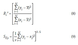
where R_iis the multiple-correlation coefficient for an equation with i independent variables, S_Eyis the standard error of estimate, x_iis the observed value (dependent variable), x is the mean of observed values (dependent variables), y_iis the estimated value of dependent variable X_i, i is the number of independent variables, N is the number of observations (sample size), and v is the degrees of freedom (AM with y-intercept = 0)

Assessment and comparison of ARFs

The derived ARF algorithms were compared to a selection of ARF estimation methods currently recommended for general use in South Africa (Pietersen et al 2015), e.g. Van Wyk (1965; Equation 10), Wiederhold (1969; Equation 11) and Alexander (2001; Equation 12) by considering six gauged catchments located in the pilot study area. Typically, the key attributes of the six gauged catchments include: (i) catchment area (30 km²< A < 2 500 km²), (ii) critical storm duration (1-h < D < 24-h), (iii) return period (10-year < T < 200-year), and (iv) MAP ranging between 430 mm and 565 mm.

where ARF_VW ARF_Wand ARF_Aare the areal reduction factors (%) as derived using the methodologies used by Van Wyk (1965), Wiederhold (1969) and Alexander (2001), A is the catchment area (km²), D is the storm duration (hours), and I_Tis the rainfall intensity (mirth^-1) based on the average design point rainfall depth (P_T).

 

RESULTS AND DISCUSSION

Analysis and disaggregation of fixed interval rainfall

The number of daily rainfall stations used (N_s), the minimum number of rainfall stations required (N_x) based on the Siriwardena and Weinmann (1996) criteria (cf, Section: Study area), observed (R₀), infilled (Rj) and total (R_t) record lengths, and corresponding percentage of infilling applicable to each quaternary catchment are summarised in Table 1 (page 24).

 

 

It is evident from Table 1 that the number of rainfall stations used (N_s) exceeds the minimum number of rainfall stations required (N_x) in each quaternary catchment, On average, the number of rainfall stations used exceeded the Siriwardena and Weinmann (1996) criteria by a ratio of 2,6, while the individual ratios varied between 1,2 and 4, These results confirm that the overall distribution and location of the daily rainfall stations are uniform and sufficient for the purpose of this study, In Table 1, the observed rainfall data represents 15 791 years, as opposed to the 6 053 infilled years, meaning that 72,3% of the total record lengths is based on observed data, At a quaternary catchment level, the percentage of infilling varied between 18,1% (C52H) and 36,7% (C51H), respectively, The latter high percentage of infilling in QC C51H could be ascribed to a large percentage of missing data, and as a result more extension was required to match the record length of the other surrounding rainfall stations. Overall, the rainfall data infilling process was carefully interrogated, and infilling was limited to periods within the observed record length under consideration, i,e, no backward extrapolation of the observed record in time, The Thiessen polygons used to convert the fixed interval observed point and areal rainfall at each rainfall station into average catchment rainfall values are shown in Figure 3.

 

 

A typical example of the fixed interval rainfall values converted and scaled to K-hour catchment rainfall using the Adamson (1981) conversion and average Smithers and Schulze (2003) scaling factors, respectively, are shown in Figure 4.

 

 

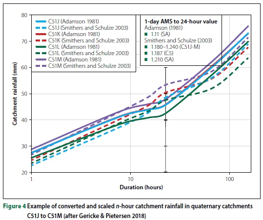
It is quite evident from Figure 4 that the converted and scaled averaged catchment rainfall for durations < 24-h tend to follow the same trend, Overall, in most of the quaternary catchments under consideration, the converted catchment rainfall values steeply increase up to 8 hours, whereafter a flatter and constant increasing slope is evident, In contrast, the scaled catchment rainfall values are characterised by an ever-increasing slope, with a notable flattening of the slope followed by an increased slope between 8-h and 24-h, For long durations > 24-h, both the converted and scaled catchment rainfall values tend to increase at a constant rate, although the converted catchment rainfall values are generally higher (Gericke & Pietersen 2018).

Probabilistic analysis of point and areal rainfall

An example of the probabilistic analyses results for both the average design point and areal design rainfall values for D = 24-h at 10-year ascending record length increments in quaternary catchment C51M is listed in Table 2 (page 25).

 

 

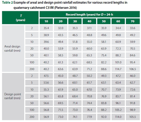
Generally, the results in Table 2 are characterised by a high variability, especially for record lengths < 30 years. Both the design point and areal design rainfall values are more consistent for longer record lengths. For instance, the variation between point and areal values for any return period is less significant with an increase in record length. Hence, this also supports the use of a minimum infilled record length of 30 years for the probabilistic analyses. A typical example of the probabilistic plot results based on the ranked point AMS values in quaternary catchment C51M for D = 24-h is illustrated in Figure 5.

 

 

In Figure 5, the probability distribution estimates proved to be comparable for return periods < 20 years; however, differences of up to 20% were evident at T = 200-year, Overall, the estimates based on the GEV/LM probability distribution proved to be statistically robust with respect to sampling variability when ARFs or design rainfall values need to be estimated and was therefore used in all 23 quaternary catchments. The latter results are also in agreement with other studies, e.g. Siriwardena and Weinmann (1996), Smithers and Schulze (2000a), Dyrrdal et al (2016) and Peleg et al (2018).

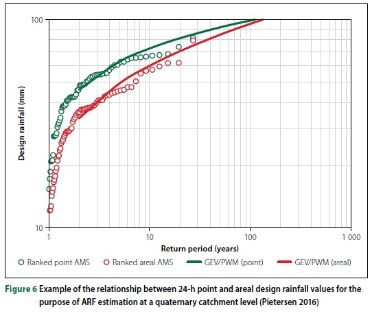
Estimation of areal reduction factors

Figure 6 is an example of the typical relationship between average design point and areal design rainfall values at a quaternary catchment level, By applying Equation 7, geographically centred and probabilistically correct ARF sample values could be obtained from Figure 6, as shown in Figure 7, In Figure 7 it is evident that the ARFs are the same for durations less than 24-h, since both the point and areal rainfall were scaled from the 1-day values using the same scaling technique having similar scaling parameters and/or statistics in a particular rainfall cluster as identified and proposed by Smithers and Schulze (2003). As an alternative, and to address these ARF values being similar for durations < 24-h, accumulated continuous measures of K-hour (short duration) rainfall data should be used.

 

 

 

 

The ranges of ARF variability at tertiary catchment levels C51 and C52 are shown in Figures 8a and 8b, respectively.

 

 

 

 

In considering Figures 7 to 8b it is clearly evident that the ARFs are not constant and tend to increase with both an increase in return period and storm duration. In both tertiary catchments C51 (Figure 8a) and C52 (Figure 8b) the ARF values range between 58% (T = 2-year; D < 24-h) and 100% (T = 100-year; D > 72-h), However, in quaternary catchments C51C, D, K and L, and C52D and F, the ARF values exceeded unity (> 100%) at T = 200-year and also tended to increase with an increase in catchment area. The latter deviation from the expected norm, i.e. ARFs decrease as the catchment size increases, could be ascribed to: (i) differences in the catchment shapes, (ii) different rainfall distribution patterns, i,e, whether storm events are aligned along the catchment or perpendicular to it, and/or (iii) the presence of uniform rainfall covering the whole catchment during higher return period events, irrespective of the catchment size under consideration. The sample ARFs, which either equalled or exceeded unity (> 100%), not only confirmed the possible presence of uniform rainfall events being associated with higher return periods (T> 100-year), but also confirmed that design point rainfall estimates are only representative of a limited area. As highlighted before, the above ARFs from individual quaternary catchments were pooled together to produce sample ARFs for a combination of catchment areas, storm durations, return periods and MAP values at a tertiary catchment level, i.e. C51 and C52. Consequently, these pooled sample ARF values served as criterion variables during the derivation of the ARF algorithms.

 

Derivation of regressions to estimate ARFs

Backward stepwise multiple linear regression analyses with deletion at a 95% confidence level resulted in the best prediction model for ARFs at a catchment level. All the independent predictor variables initially considered, e.g. A, T, D and MAP were retained and included in the calibrated equation(s) applicable to each tertiary drainage region. Hence, the same equation format (Equation 13), with different regional calibration coefficients (Table 3), was used in C51 and C52, respectively.

 

 

 

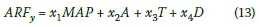
where ARF_yis the estimated ARF (%), A is the catchment area (km²), D is the storm duration (hours), MAP is the mean annual precipitation (mm), T is the return period (years), and x₁ to x₄ are the regional calibration coefficients (Table 3).

In considering the GOF statistics and hypothesis testing results, as listed in Table 4, it is evident that the best results were obtained in the C52 tertiary drainage region, with the standard error of the ARF_yestimate = 6,6% and an associated coefficient of multiple-correlation = 0,85.

 

 

Scatter plots of the ARF_T(Equation 7) and ARF_y(Equation 13) values associated with all the quaternary catchments in each tertiary drainage region are shown in Figure 9 to highlight any regional differences, In Figure 9, the ARF_yvalues computed using Equation 13 displayed a low to moderate degree of association with the ARF_Tvalues (Equation 7), with r² values ranging between 0,2 (C51) and 0,5 (C52).

 

 

Such low r²values are not only indicative of a low degree of association, but also highlight the heterogeneity between ARFs in different quaternary catchments due to the non-uniform rainfall distribution. The latter influence of non-uniform rainfall distribution on the ARF estimates was confirmed by the estimation of individual r²values at a quaternary catchment level. Typically, the r²values ranged from 0,48 ~ 0,80, thus confirming that the rainfall distribution is more uniform over a smaller geographically fixed area.

However, in the C51 tertiary drainage region, it is clearly evident that the ARF_yvalues (Equation 13) are quite sensitive to MAP variability, especially for MAP values beyond the calibration range, i.e. values lower and higher than the minimum (326 mm) and maximum (576 mm) MAP values used during the calibration process. In addition, factors that might have an influence on the degree of association between the ARF_T(Equation 7) and ARF_y(Equation 13) values in the 23 quaternary catchments are: (i) catchment shape, (ii) geographical cen-tredness of ARF estimates, (iii) orientation, direction and spatial extent of non-uniform rainfall not covering the whole catchment, and (iv) potential rainfall data quality discrepancies. Overall, the above results confirmed that ARFs vary with catchment area, storm duration, return period and MAP.

Assessment and comparison of ARFs

The ARF estimates based on Equations 10 to 13 in the six gauged catchments located in the pilot study area are summarised in Table 5. In comparing the ARF estimates, a number of notable trends are evident from Table 5.

 

 

In catchment areas (A) < 1 000 km², the ARF_VWestimates based on Equation 10 (Van Wyk 1965) tend to be nearly constant and vary between 91% and 97%. In catchment areas (A) > 1 000 km², the ARF values decrease with an increase in catchment area, storm duration and return period, The ARF_Westimates based on Equation 11 (Wiederhold 1969) also decreased with an increase in both catchment area and storm duration, while they remained constant for the various return periods, It is important to note that both Equations 10 and 11 are storm-centred approaches, which are essentially not suitable to estimate the catchment areal design rainfall from design point rainfalls. In doing so, the practitioner would by default incorrectly assume that extreme design point rainfall and extreme areal design rainfall are produced by the same rainfall event or rainfall type. As in the case of Equation 11, the ARF_Aestimates based on Equation 12 (Alexander 2001) also decreased with an increase in both catchment area and storm duration, while being constant for the various return periods. However, Equation 12 resulted in ARF_Aestimates that are between 15% and 27% higher, The latter differences also tend to decrease with an increase in both catchment area and storm duration.

In contrast, the ARF_yestimates based on Equation 13 (this study) increased with an increase in catchment area, storm duration and return period, except in catchment C5H054 where the ARFs tend to be lower than those ARFs estimated in the smaller catchments, The latter increase of ARFs with an increase in catchment area, storm duration and return period is also in agreement with the trends witnessed in the design rainfall values (cf. Section: Estimation of areal reduction factors) used to estimate the observed' ARFs (Equation 7). On average, the ARF estimates based on Equations 10 to 13 differed from one another with between 4% and 26%, with smaller differences associated with higher return periods. The highest individual differences, up to 31%, are evident between the storm-centred approaches, i,e, Equations 10 and 11, but the differences also decreased with an increasing return period. The highest degree of association is evident between Equations 10 and 12, with differences limited to 8%.

However, Equation 10 varies with the return period, while Equation 12 remains constant irrespective of the return period under consideration.

Based on the above results, it is evident that the storm-centred approaches, which resulted in lower ARFs associated with higher return periods, are unable to represent the spatial and temporal distribution of severe storm mechanisms (T > 50-year) that produce high-intensity rainfall with cell core areas exceeding the areal range and storm duration under consideration. Furthermore, constant ARF values associated with variable return periods, e.g. Equations 11 and 12, are regarded as probabilistically incorrect, Hence, despite the fact that the ARF estimates based on Equation 13 increased with an increase in catchment area, it is the only method that could be regarded as probabilistically correct, i.e. ARFs increased with both an increase in return period and storm duration. The latter also confirmed that the current ARF methodologies used in South Africa are only applicable to specific temporal and spatial scales.

 

CONCLUSIONS

In this paper, an improved methodology to express the spatial and temporal rainfall variability at a quaternary catchment level by means of geographically centred and probabilistically correct ARFs was developed. The ARF values obtained are regarded as being probabilistically correct since the relationships between average areal design rainfall and average design point rainfall estimates for various catchment areas, storm durations, return periods and MAP values at a catchment level were established, The major findings could be summarised as follows:

a. Design point rainfall estimates are only representative of a limited area, In larger catchment areas the average areal design rainfall depth is likely to be less than the maximum design point rainfall depths, except in cases where uniform rainfall events covering the whole catchment area are associated with higher return periods (T > 100-year).

b. ARFs are not constant and vary with catchment area, storm duration, return period and MAP, In applying Equation 7 to the geographically centred and probabilistic ARF sample values obtained from the observed daily rainfall data, the ARF values increased with both an increase in return period and storm duration, However, in some quaternary catchments, the ARF values exceeded unity (> 100%) at T = 200-year, and also tended to increase with an increase in catchment area.

c. Estimated ARF values that increase with an increase in catchment area could mainly be ascribed to differences in catchment shape and the orientation, direction and spatial extent of rainfall events in relation to the catchment area under consideration.

d. The geographically centred approach based on a modified version of Bell's method has proved to be appropriate for the pilot study undertaken and bounded within a 'fixed' catchment area, i,e, the C5 secondary drainage region.

e. The derived algorithm(s) (Equation 13) provided improved probabilistic ARF estimates in comparison to the geographically and storm-centred methods currently used in South Africa.

f. The current South African ARF methodologies (Equations 10 - 12) are only applicable to specific temporal and spatial scales and do not account for any regional differences, Only Equation 10 is regarded as being probabilistically correct, i.e. ARFs vary with return period. However, both Equations 10 and 11 are storm-centred approaches which are currently generally incorrectly applied by practitioners in a geographically centred manner, Furthermore, Equation 12 is the only geographically centred method currently used in South Africa, although it was transposed from methods developed in the United Kingdom with little local verification and is also regarded as being probabilistically incorrect, since the ARF estimates remain constant irrespective of the return period under consideration.

Conversely, in view of the results obtained from this study, especially as shown in Figure 9, it is also evident that the methodology used in this study need to be reinvestigated and expanded to other catchments in South Africa and/or internationally by incorporating: (i) the use of circular test catchments as opposed to actual catchments (with a unique shape, orientation and size) to eliminate the impact of catchment size and shape on rainfall distribution patterns, (ii) the further refinement, calibration and verification of the derived ARF algorithms at a circular catchment level, (iii) the regionalisation of the ARF algorithms, (iv) the estimation of ARF index values to enable the transfer of hydrological information from gauged to ungauged sites, and (v) the development of a software interface to enable practitioners to apply and use the regionalised ARF algorithms, The incorporation of the above-listed steps towards the estimation of probabilistically correct ARFs are warranted to eliminate the current shortcomings experienced.

At a national level, it is envisaged that the implementation and expansion of both the identified research values, adopted methodology and recommendations for future research will contribute towards improved ARF estimations using a geographically centred approach, Fortunately, the additional research conducted by Du Plessis et al (2020) on radar-based storm-centred ARFs in South Africa is almost completed, with radar imagery from SAWS and the North West University (NWU) being used to compile 1-, 3- and 24-h design rainfall information to derive storm-centred ARFs, Consequently, these updated geographically centred and/or storm-centred approaches to ARF estimation will ultimately contribute towards improved design flood estimations

 

ACKNOWLEDGEMENTS

Support for this research by the Central University of Technology, Free State (CUT), National Research Foundation (NRF) and Water Research Commission (WRC) is gratefully acknowledged, We also wish to thank the anonymous reviewers for their constructive review comments, which have helped to significantly improve the paper.

 

REFERENCES

Adamson, P T 1981. Southern African storm rainfall. Technical Report TR102. Pretoria: Department of Environmental Affairs and Tourism.         [ Links ]

Alexander, W J R 2001. Flood risk reduction measures: Incorporating flood hydrology for Southern Africa. Pretoria: University of Pretoria, Department of Civil and Biosystems Engineering.         [ Links ]

Allen, R J & De Gaetano, A T 2005. Areal reduction factors for two eastern United States regions with high rain-gauge density. Journal of Hydrologie Engineering, 10(4): 327-335.         [ Links ]

Asquith, W H & Famiglietti, J S 2000. Rainfall areal reduction factor estimation using annual-maxima centered approach. Journal of Hydrology, 230(1-2): 55-69.         [ Links ]

Bacchi, B & Ranzi, R 1996. On the derivation of the areal reduction factor of storms. Atmospheric Research, 42:123-135.         [ Links ]

Bell, F C 1976. The areal reduction factor in rainfall frequency estimation. Report No. 35. London; Natural Environment Research Council, Institute of Hydrology.         [ Links ]

Bengtsson, L & Niemczynowicz, J 1986. Areal reduction factors from rain movement. Nordic Hydrology 17(2): 65-82.         [ Links ]

De Michéle, C, Kottegoda, N T & Rosso, R 2001. The derivation of areal reduction factor of storm rainfall from its scaling properties. Water Resources Research, 37(12): 3247-3252.         [ Links ]

Du Plessis, J A, Burger, R P, Gericke, O J, Thomas, T J and Marebane, T S 2020. The applicability of the use of radar data to develop areal reduction factors in South Africa. WRC Report No. K5-2923. Pretoria: Water Research Commission.         [ Links ]

DWAF (Department of Water Affairs and Forestry) 1995. GIS data: Drainage regions of South Africa. Pretoria: DWAF.         [ Links ]

Dyrrdal, A V, Skaugen, T, Stordal, F & Forland, E J 2016. Estimating extreme areal precipitation in Norway from a gridded dataset. Hydrological Sciences Journal, 61(3): 483-494.         [ Links ]

Eggert, B, Berg, P, Haerter, J O, Jacob, D and Moseley, C 2015. Temporal and spatial scaling impacts on extreme precipitation. Atmospheric Chemistry and Physics, 15(10): 5957-5971.         [ Links ]

Gericke, O J & Du Plessis, J A 2011. Evaluation of critical storm duration rainfall estimates used in flood hydrology in South Africa. Water SA, 37(4): 453-470. DOT 10.4314/wsa.v37i4.4.         [ Links ]

Gericke, O J & Smithers, J C 2014. Review of methods used to estimate catchment response time for the purpose of peak discharge estimation. Hydrological Sciences Journal, 59(11): 1935-1971. DOI: 10.1080/02626667.2013.866712.         [ Links ]

Gericke, O J & Pietersen, J P J 2018. Disaggregation of fixed time interval rainfall to continuous measured rainfall for the purpose of design rainfall estimation. Water SA, 44(4): 557-568. DOT 10.4314/wsa.v44i4.05.         [ Links ]

Grebner, G & Roesch, T 1997. Regional dependence and application of DAD relationships. International Association of Hydrological Sciences, 246: 223-230.         [ Links ]

Kim, J, Tee, J, Kim, D & Kang, B 2019. The role of rainfall spatial variability in estimating areal reduction factors. Journal of Hydrology, 568:416-426.         [ Links ]

Li, J, Sharma, A, Johnson, F & Evans, J 2015. Evaluating the effect of climate change on areal reduction factors using regional climate model projections. Journal of Hydrology, 528: 419-434.         [ Links ]

Tynch, S D 2004. Development of a raster database of annual, monthly and daily rainfall for Southern Africa. WRC Report No. 1156/1/04. Pretoria: Water Research Commission.         [ Links ]

McCuen, R H 2005. Hydrologie Analysis and Design, 3rd ed. New York: Prentice-Hall.         [ Links ]

Midgley, D C, Pitman, W V & Middleton, B J 1994. Surface water resources of South Africa. Volume 2, Drainage Region C, Vaal: Appendices. WRC Report 298/2.1/94. Pretoria: Water Research Commission.         [ Links ]

Mineo, C, Ridolfi, E, Napolitano, F & Russo, F 2018. The areal reduction factor: A new analytical expression for the Tazio Region in central Italy. Journal of Hydrology, 560: 471-479.         [ Links ]

NERC (Natural Environment Research Council) 1975. Flood studies report. Tondon: NERC.         [ Links ]

Pavlovic, S, Perica, S, St Taurent, M & Mejia, A 2016. Intercomparison of selected fixed-area areal reduction factor methods. Journal of Hydrology, 537: 419-430.         [ Links ]

Peleg, N, Marra, F, Fatichi, S, Paschalis, A, Moinar, P & Burlando, P 2018. Spatial variability of extreme rainfall at radar subpixel scale. Journal of Hydrology, 556: 922-933.         [ Links ]

Pietersen, J P J, Gericke, O J, Smithers, J C & Woyessa, Y E 2015. Review of current methods for estimating areal reduction factors applied to South African design point rainfall and preliminary identification of new methods. Journal of the South African Institution of Civil Engineering, 57(1): 16-30.         [ Links ]

Pietersen, J P J 2016. Areal reduction factors for design rainfall estimation in the C5 secondary drainage region of South Africa. Unpublished MTech Eng. Dissertation. Bloemfontein: Central University of Technology, Free State.         [ Links ]

Podger, S, Green, J, Stensmyr, P & Babister, M 2015. Creating long duration areal reduction factors, Proceedings, 36th Hydrology and Water Resources Symposium: The Art and Science of Water, Hobart, Australia, pp. 210-219.         [ Links ]

SANRAL (South African National Roads Agency Limited) 2013. Drainage Manual, 6th ed. Pretoria; SANRAL.         [ Links ]

Singh, S K, Griffiths, G A & McKerchar, A I 2018. Towards estimating areal reduction factors for design rainfalls in New Zealand. Journal of Hydrology (New Zealand), 57(1): 25-33.         [ Links ]

Siriwardena, L & Weinmann, P E 1996. Derivation of areal reduction factors for design rainfalls in Victoria. Report No. 96/4. Victoria, Australia; Cooperative Research Centre for Catchment Hydrology.         [ Links ]

Sivapalan, M & Bloschl, G 1998. Transformation of point rainfall to areal rainfall: Intensity-duration-frequency curves. Journal of Hydrology, 204(1-4): 150-167.         [ Links ]

Skaugen, T 1997. Classification of rainfall into small- and large-scale events by statistical pattern recognition. Journal of Hydrology, 200(1-4): 40-57.         [ Links ]

Smithers, J C & Schulze, R E 2000a. Development and evaluation of techniques for estimating short duration design rainfall in South Africa. WRC Report No. 681/1/00. Pretoria: Water Research Commission.         [ Links ]

Smithers, J C & Schulze, R E 2000b. Long duration design rainfall estimates for South Africa. WRC Report No. 811/1/00. Pretoria: Water Research Commission.         [ Links ]

Smithers, J C & Schulze, R E 2003. Design rainfall and flood estimation in South Africa. WRC Report 1060/01/03. Pretoria: Water Research Commission.         [ Links ]

Smithers, J C & Schulze, R E 2004. The estimation of design rainfall for South Africa using a regional scale invariant approach. Water SA, 30(4): 435-444.         [ Links ]

Stewart, E J 1989. Areal reduction factors for design storm construction: Joint use of rain gauge and radar data. Association of Hydrological Sciences, 181: 31-40.         [ Links ]

Svensson, C & Jones, D A 2010. Review of methods for deriving areal reduction factors. Journal of Flood Risk Management, 3(2010): 232-245.         [ Links ]

USGS (United States Geological Survey) 2016. EarthExplorer. https://earthexplorer.usgs.gov (accessed on 19 September 2016).         [ Links ]

USWB (United States Weather Bureau) 1957. Rainfall intensity-frequency regime, the Ohio Valley. Technical Paper 29. Washington, DC: USWB.         [ Links ]

USWB 1958. Rainfall intensity-frequency regime, south-eastern United States. Technical Paper 29. Washington, DC: USWB.         [ Links ]

Van Wyk, W 1965. Aids to the prediction of extreme floods from small watersheds. Johannesburg; University of the Witwatersrand, Department of Civil Engineering.         [ Links ]

Wiederhold, J F A 1969. Design storm determination in South Africa. HRU Report No. 1/1969. Johannesburg: University of the Witwatersrand, Hydrological Research Unit.         [ Links ]

Wilson, E M 1990. Engineering Hydrology, 4th ed. London: Macmillan.         [ Links ]

 

 

Correspondence:
Prof Jaco Gericke
Department of Civil Engineering, Faculty of Engineering, Built Environment and Information Technology, Central University of Technology, Free State
Bloemfontein, South Africa
T: +27 51 507 3516
E: jgericke@cut.ac.za

Jaco Pietersen
Department of Civil Engineering, Faculty of Engineering, Built Environment and Information Technology, Central University of Technology, Free State
Bloemfontein, South Africa
T: +27 51 507 3693
E: jpietersen@cut.ac.za

 

 

 

PROF JACO GERICKE Pr Eng, IntPE (SA), is the Head of Department (Civil Engineering) at the Central University of Technology, Free State. He obtained his PhD Eng (Agriculture) degree from the University of KwaZulu-Natal in 2016 and has more than 20 years' professional and academic experience, mainly in the fields of hydrology, water resources management and river hydraulics. He has published a number of papers in the design hydrology field and is currently involved in four research projects funded by the Water Research Commission.

 

 

JACO PIETERSEN Pr Tech Eng is currently employed by the Central University of Technology, Free State (CUT). He graduated with B Tech Eng (Civil) and M Tech Eng (Civil) degrees from the CUT and has a special interest in flood hydrology and water resources management. In addition to his ten years' academic experience, he also worked at an internationally recognised civil engineering consultancy for five years. He is currently studying towards a D Eng (Civil) degree at the CUT.