TECHNICAL PAPER

 

A case for the adoption of decentralised reinforcement learning for the control of traffic flow on South African highways

 

 

T Schmidt-Dumont; J H van Vuuren

Correspondence

 

 

---

ABSTRACT

As an alternative to capacity expansion, various dynamic highway traffic control measures have been introduced. Ramp metering and variable speed limits are often considered to be effective dynamic highway control measures. Typically, these control measures have been employed in conjunction with either optimal control methods or online feedback control. One shortcoming of feedback control is that it provides no guarantee of optimality with respect to the chosen metering rate or speed limit. Optimal control approaches, on the other hand, are limited in respect of their applicability to large traffic networks due to their significant computational expense. Reinforcement learning is an alternative solution approach, in which an agent learns a near-optimal control strategy in an online manner, with a smaller computational overhead than those of optimal control approaches. In this paper an empirical case is made for the adoption of a decentralised reinforcement learning approach towards solving the control problems posed by both ramp metering and variable speed limits simultaneously, and in an online manner. The effectiveness of this approach is evaluated in the context of a microscopic traffic simulation model of a section of the N1 national highway outbound from Cape Town in South Africa's Western Cape Province.

Keywords: ramp metering, variable speed limits, reinforcement learning, highway traffic control, traffic simulation

---

 

 

INTRODUCTION

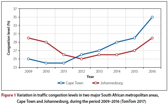
Highways were originally built with the aim of providing virtually unlimited mobility to road users. The ongoing dramatic expansion of car ownership and travel demand has, however, led to the situation where, today, traffic congestion is a significant problem in major metropolitan areas all over the world (Schranck et al 2012). The reason for the severe traffic congestion experienced around the world is over-utilisation of the existing road infrastructure which potentially leads to dense, stop-and-go traffic. Although traffic congestion is typically associated with well-developed countries such as the United States, China or Germany, it is also a major problem in South Africa. According to the TomTom Traffic Index (TomTom 2017), a congestion ranking based on GPS data collected from individual vehicles, Cape Town is the 48^th most congested city in the world, and the most congested city in Africa. In order to place these statistics into perspective, Cape Town has the same congestion ranking as New York City according to the TomTom Traffic Index published at the end of 2016. The morning and afternoon peak congestion in Cape Town furthermore exceeds that experienced by commuters in New York City.

Traffic congestion levels in Cape Town have increased steadily since 2011, with a significant increase in congestion levels from 30%% in 2015 to 35%% in 2016 (TomTom 2017). These percentages imply that a journey would have taken, on average, 35% longer in 2016 due to congestion than it would have taken if free-flowing traffic conditions had prevailed. During the morning and afternoon peaks, the levels of traffic congestion are naturally higher than these average values suggest. Travellers experience a 75% increase in travel time during the morning peak, while commuters experience a 67% increase in travel time during the afternoon peak. The result of these levels of traffic congestion is that the average Capetonian spends an additional 42 minutes stuck in traffic per day, which accumulate to approximately 163 hours stuck in traffic per year (TomTom 2017).

In Figure 1 it is shown that congestion levels in Johannesburg temporarily decreased from 2009 to 2012. This decrease may be attributed to capacity expansion as a result of the Gauteng Freeway Improvement Project (SANRAL 2009). The subsequent rise in congestion levels during the period 2012-2016, visible in the figure, may be attributed to the so-called theory of induced traffic demand, in which it is suggested that increases in highway capacity will induce additional traffic demand, thus not permanently alleviating congestion as envisioned (Noland 2001).

 

 

The alternative to capacity expansion aimed at improving traffic flow on highways is more effective control of the existing infrastructure. Ramp metering (RM) is a means of improving highway traffic flow through effective regulation of the flow of vehicles that enter a highway traffic flow from an on-ramp. In this way, the mainline throughput may be increased due to an avoidance of capacity loss and blockage of on-ramps as a result of congestion (Papageorgiou & Kotsialos 2000). Variable speed limits (VSLs) were initially employed mainly with the aim of improving traffic safety on highways due to the resulting homogenisation of traffic flow (Hegyi et al 2005). In more recent developments, however, VSLs have been employed as a traffic flow optimisation technique with the aim of improving traffic flow along highways. This improvement may take one of two forms, either maintaining stable traffic flow by slightly reducing the speed limit in order to reduce the differences in speed between vehicles and reduce the following distance, resulting in improved traffic flow (Hegyi et al 2005), or by decreasing the speed limit to such an extent that an artificial bottleneck is created, inducing controlled congestion, but maintaining free-flow traffic at the true bottleneck location (Carlson et al 2010). RM and VSLs are considered to be effective highway traffic control measures (Papageorgiou & Kotsialos 2000). An empirical case is made in this paper for their adoption within a South African context. Traditionally, classical feedback control theory has been employed in the design of controllers for implementing RM and VSLs (Carlson et al 2014). One drawback of the classical feedback control approach is that it provides no guarantee of optimal control. Furthermore, feedback controllers are purely reactive, which may result in delayed response.

Reinforcement learning (RL) provides a promising framework addressing these issues. The objective in this paper is to compare, for the first time, the relative effectiveness of state-of-the-art feedback controllers from the literature with that of employing a decentralised RL approach towards solving the RM and VSL problems simultaneously in the context of a real-world scenario. Furthermore, this paper contains, to our best knowledge, the first application of multi-agent reinforcement learning (MARL) approaches at several consecutive on-ramps contained within the same simulation model.

 

LITERATURE REVIEW

In this section a review of RM and VSL controllers from literature is provided, followed by a brief introduction to RL.

Highway traffic control measures

Wattleworth (1967) introduced the first RM strategies, which were based on historical traffic demand at on-ramps, setting specific metering rates for certain time intervals in order to control the inflow of traffic onto the highway. In search of a more adaptive RM strategy, Papageorgiou et al (1991) introduced the well-known Asservissement Lineaire d'entrée Autoroutiere (ALINEA) control mechanism, which is based on online feedback control theory. An extension of the ALINEA control strategy, called PI-ALINEA, was later introduced by Wang et al (2014) such that bottlenecks occurring further downstream than the immediate lane merge may also be taken into account. Alternative existing RM solutions include a model predictive control (MPC) approach proposed by Hegyi et al (2005) and an implementation of a hierarchical control approach by Papamichail et al (2010). Early RM approaches, however, often led to the formation of long queues of vehicles building up on the on-ramp, which may cause congestion in the arterial network. This issue was addressed by Smaragdis and Papageorgiou (2003) who designed an extension to be implemented in conjunction with a feedback controller (such as ALINEA) which, in cases of severe congestion, maintains a maximum on-ramp queue length set to some pre-specified value. A second metering rate is calculated, ensuring the maximum allowable queue length is not exceeded, and the least restrictive metering rate is then applied (Smaragdis & Papageorgiou 2003).

An early attempt at employing RL to solve the RM problem with the aim of learning optimal control policies in an online manner is due to Davarjenad et al (2011). They employed the well-known Q-Learning RL algorithm (Watkins & Dayan 1992) in order to learn optimal metering rates within the context of a macroscopic traffic simulation model developed in the well-known METANET traffic modelling software, while simultaneously considering the buildup of on-ramp queues. Rezaee et al (2013) demonstrated the first application of RL for solving the RM problem in the context of a microscopic traffic simulation model, in which a portion of Highway 401 in Toronto, Canada was considered.

Smulders (1990) demonstrated one of the first applications of VSLs as an optimisation technique. In his formulation of the VSL control problem as an optimal control problem, which was based on a macroscopic traffic simulation model, the aim was to determine speed limits such that the expected time until traffic congestion occurs is maximised. Alessandri et al (1998, 1999) later on extended and refined this original optimal control approach. Carlson et al (2011) subsequently proposed an online feedback controller. The controller receives real-time traffic flow and density measurements as input, which are subsequently used to calculate appropriate speed limit values with the aim of maintaining stable traffic flows that are close to pre-specified reference values. In this manner, increased throughput may be achieved for various scenarios of traffic demand. A simpler version of such an online feedback controller was later introduced by Müller et al (2015).

Zhu and Ukkusuri (2014), as well as Walraven et al (2016), have shown that the VSL problem may be solved using RL techniques. Zhu and Ukkusuri (2014) demonstrated an application of the R-Markov Average Reward Technique (R-MART) RL algorithm for solving the VSL control problem within the context of a macroscopic link-based dynamic network loading model. Walraven et al (2016), on the other hand, employed Q-Learning in conjunction with a neural network for function. In both the studies mentioned above, the VSL problem was addressed within a macroscopic traffic modelling paradigm. This paradigm may, however, be limiting as it is often difficult to replicate some of the important, realistic characteristics of traffic flow, including shockwave propagation, or the spill-back effect which may occur due to heavy congestion (Zhu & Ukkusuri 2014).

Carlson et al (2014) proposed an integrated feedback controller for simultaneously performing both RM and enforcing VSLs. This controller comprises two individual feedback controllers. The RM controller operates according to the PI-ALINEA feedback controller with the addition of the queue limitation as defined by Smaragdis and Papageorgiou (2003). RM is then applied by itself until the on-ramp queue limit is reached, at which point a VSL controller, such as that of Carlson et al (2011) or Müller et al (2015), is employed in order to provide supplementary highway traffic flow control.

In the RL implementations for RM and VSLs mentioned above, the RL approaches were typically able to outperform the corresponding feedback controllers (Rezaee et al 2013; Walraven et al 2016). RL has, however, not been employed for solving the RM and VSL control problems simultaneously within the context of a real-world case study. It is envisioned that a MARL approach for simultaneously employing RM and VSLs may lead to further improvements in the travel times experienced by motorists. RL followed by its implementations in this paper, working towards the MARL approach, is outlined in the following sections.

Reinforcement learning

RL is the concept of learning an optimal control policy by trial and error (Sutton & Barto 1998). A learning agent receives information about the current state of the environment in which it operates at each time step. This state of the environment is typically defined by one or a number of descriptive state variables. Based on this state information, the agent performs an action that subsequently transforms the environment in which it finds itself into a new state. An agent's behaviour is defined by its policy, which is the mapping according to which the agent chooses its action based on the current state information. The agent receives feedback in the form of a scalar reward so as to provide it with an indication of the quality of the action chosen. This reward is typically determined based on the new state of the environment, according to a specific reward function. The aim of an RL agent is to learn a policy according to which the accumulated reward that it receives over time is maximised (i.e. finding a policy that results in the agent choosing the best action in each state with respect to the long-term cumulative reward achieved) (Szepesvari 2010).

 

REINFORCEMENT LEARNING IMPLEMENTATIONS

Reinforcement learning for RM

Davarjenad et al (2011) and Rezaee et al (2013) demonstrated that RL techniques may be employed for solving the RM problem. RM is typically enforced by a traffic signal located at an on-ramp, employing a one-vehicle-per-green-phase metering protocol (Hegyi et al (2005). The traffic signal is thus given a fixed green phase time of three seconds, allowing a single vehicle to pass during every green phase, while the RL agent controls the red phase times, thereby regulating the flow of vehicles allowed to join the highway traffic flow. An RL agent is thus required to control the traffic light at each on-ramp where RM is enforced.

The state space

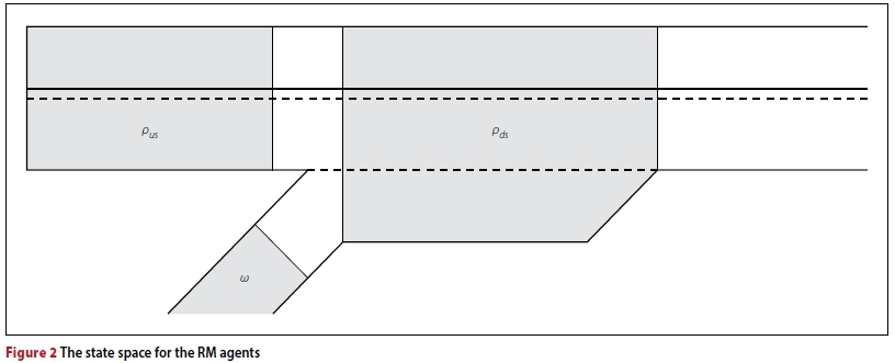
As may be seen in Figure 2, the state space of the RM agent comprises three variables. The first of these is the density ρ_dsmeasured directly downstream of the on-ramp. It is expected that this variable will provide the agent with explicit feedback in respect of the quality of the previous action, because the merge of the on-ramp and highway traffic flows is expected to be the source of congestion. Therefore, the downstream den sity is expected to be the earliest indicator of impending congestion. The density p_us measured upstream of the on-ramp is the second state variable. The upstream density is included in the state space, because it provides information on the propagation of congestion backwards along the highway.

The on-ramp queue length w is the third state variable, which was included to provide the learning agent with an indication of the on-ramp demand.

The action space

Based on the current state of traffic flow on the highway, the learning agent may select a suitable action. In this study, direct action selection (i.e. directly choosing a red phase duration from a set of pre-specified red times) is applied. As in the implementation of Rezaee et al (2013), the agent may choose an action a ε {0, 2, 3, 4, 6, 8, 10, 13}, where each action represents a corresponding red phase duration in seconds. Assuming a fixed green phase duration of three seconds, as stated above, these red phase durations result in on-ramp flows of q₀R ε {1650, 720, 600, 514, 400, 327, 277, 225} vehicles per hour, given sufficient on-ramp demand.

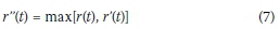
The reward function

When designing a traffic control system, the typical objective is to minimise the total travel time spent in the system by all transportation users. From the fundamental theory of traffic flow it follows that maximum throughput occurs at the critical density of a specific highway section (Papageorgiou & Kotsialos 2000). Therefore, an RM agent typically aims to control the density on the highway. This is the case in ALINEA, the most celebrated RM technique (Rezaee et al 2013). The reward function employed in this paper was inspired by the ALINEA control law. According to the ALINEA control strategy, the metering rate employed at an on-ramp is adjusted based on the difference between a desired downstream density and the measured downstream density (Papageorgiou et al 1991). Furthermore, an additional punishment is included in the reward function to refrain the agent from enforcing metering rates which lead to the build-up of long on-ramp queues. The reward of the RM RL agents is therefore calculated as:

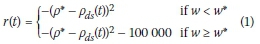
where ρ* denotes the desired downstream density that the RL agent aims to achieve, while p_ds(t) denotes the actual downstream density measured during the last control interval, t, w denotes the current measured on-ramp queue length, and w* denotes the maximum allowable on-ramp queue length. In order to provide amplified negative feedback to the agent for actions that result in large deviations from the target density, this difference is squared. Both the Q-Learning (Watkins & Dayan 1992) and /NN-TD learning (Martin et al 2011) algorithms are implemented for RM in this paper.

Reinforcement learning for VSLs

Zhu and Ukkusuri (2014) and Walraven et al (2016) have demonstrated formulations of the VSL problem as RL problems, and subsequently solved these using RL algorithms. We apply VSLs in the vicinity of each of the on-ramps. The VSLs determined by the RL agent are typically enforced by displaying the current speed limit on a roadside variable message sign.

The state space

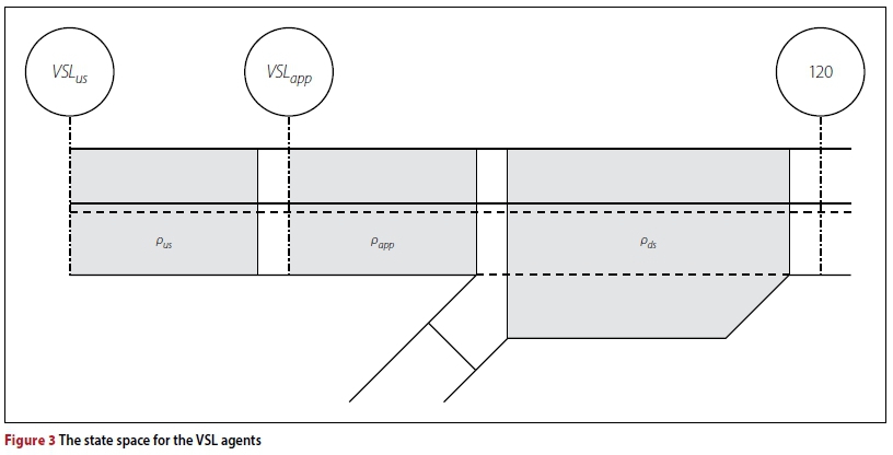
Similarly to the RM implementations, the state space for the VSL implementations comprises three variables, as shown in Figure 3. The first of these state variables is, as for the RM implementations, the density p_ds directly downstream of the on-ramp. This variable is again chosen so as to provide the VSL agent with information on the state of traffic flow at the bottleneck location. The density directly upstream of the bottleneck location, denoted by p_app, is the second state variable. This is the key focus area where a VSL is applied. It is expected that the most immediate response to an action will be reflected on this section of a highway. Therefore, this variable should provide the agent with an indication of the effectiveness of the chosen action. Finally, the third state variable is the density measured on the highway section further upstream from that comprising the area considered for the second state variable, denoted by p_us. This variable is chosen primarily to provide a predictive component in terms of highway demand. Furthermore, this variable is expected to provide the agent with an indication of the severity of the congestion in cases where it has spilled back beyond the application area of p_app^.

The action space

Similarly to the RM implementation, direct action selection is employed in the VSL implementation. We applied the VSL:

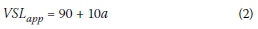
where a ε {0,1,2,3} applies. As a result, minimum and maximum variable speed limits of 90 km/h and 120 km/h respectively may be applied at the application area. The lower limit, as well as the increment of 10 km/h, was empirically determined to achieve the best performance. In order to reduce the difference in speed limit from 120 km/h to VSL_app, the speed limit at the upstream section is adjusted according to:

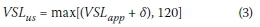
It is envisioned that this more gradual reduction in the speed limit will reduce the probability of shock-waves which may be a result of sharp, sudden reductions in the speed limit propagating backwards along the highway.

The reward function

The VSL agent also aims to minimise the total time spent in the system by all transportation users, by maximising the system throughput. Therefore, the VSL agent is rewarded according to the flow rate out of the bottleneck location, measured in veh/h. Similarly to the RM implementations, Q-Learning (Watkins & Dayan 1992) and kNN-TD learning (Martin et al 2011) are implemented for VSLs.

Multi-agent reinforcement learning for combined RM and VSLs

We also consider three approaches towards simultaneously solving the RM and VSL problems by means of multi-agent reinforcement learning (MARL) (Busoniu et al 2008). Employing independent learners (El Tantaway et al 2013) is the first and the simplest of these approaches, where both the RM and VSL agents learn independently, without any form of communication between them, as they both aim simply to maximise their own, local rewards. In the second approach, hence-forth referred to as the hierarchical MARL approach, a hierarchy of learning agents is established. Action selection is performed according to the order in this hierarchy (i.e. the agent assigned the highest rank may choose first, followed by the second-highest ranked agent, and so forth) (Busoniu et al 2008). Once the highest ranked agent has chosen its action, this action is communicated to the second-highest ranked agent. The second-highest ranked agent can then take this action into account and select its own action accordingly. As a result of this communication, the state-action space of the second agent grows by a factor equal to the number of actions available to the first agent. These rankings may be determined empirically, or in the order of performance of the individual agents. The maximax MARL approach, which is the third and most sophisticated MARL approach, is based on the principle of locality of interaction among agents (Nair et al 2005). According to this principle, an estimate of the utility of a local neighbourhood maps the effect of an agent's actions to the global value function (only the neighbouring agents are considered) (El Tantawy et al 2013). The implementation works as follows:

1. Each agent i chooses an action which is subsequently communicated to its neighbouring agent j.

2. Each agent i finds an action aⁱ_(t+1) that maximises the joint gain in rewards.

3. This joint gain is calculated for each agent i as if it were the only agent allowed to change its action, while its neighbour's action remains unchanged.

4. The agent able to achieve the largest joint gain changes its action, while the action of the neighbour remains unchanged. The process is repeated from Step 2 until no action by either agent results in an increase in the joint gain.

5. The entire process is repeated during each learning iteration.

Due to this two-way communication, the state-action space of each agent increases by a factor equal to the number of actions available to its neighbour in the maximax MARL approach. The following section is devoted to a discussion of the highway traffic simulation model in which these control measures and algorithms were implemented.

 

THE MICROSCOPIC TRAFFIC SIMULATION MODEL

In this section, a description of the microscopic traffic simulation model, which is used as the algorithmic test bed, is provided, illustrating the modelling tools employed, as well as the model calibration based on input data, and the techniques for analysis of the output data.

Modelling tools employed and case study area

A simulation model was developed as algorithmic test bed within the AnyLogic 7.3.5 University Edition (AnyLogic 2017) software suite, making specific use of its built-in Road Traffic and Process Modelling Libraries. The road traffic library allows for microscopic traffic modelling, where each vehicle is simulated individually.

The highway section modelled is a stretch of the N1 national highway outbound from Cape Town in South Africa's Western Cape Province, from just before the R300 off-ramp (denoted by O1) up to a section after the on-ramp at the Okavango Road interchange (denoted by D₃), as shown in Figure 4. Five on- and off-ramps fall within this study area, namely the off-ramp at the R300 interchange (denoted by D₁), the on-ramp at the Brackenfell Boulevard interchange (denoted by O₃), the off-ramp at the Okavango Road interchange (denoted by D₂), and the on-ramp at the Okavango Road interchange (denoted by O₄). This stretch of highway experiences significant congestion problems, especially during the afternoon peak, when large traffic volumes enter the N1 from the R300 and leave the N1 at the Okavango Road off-ramp.

 

 

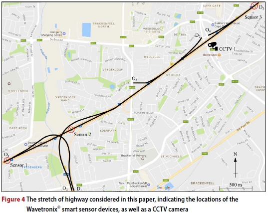
Model input data

Model input data was required for calibration and validation of the simulation model. This data was obtained from two major sources. The primary sources were Wavetronix® (Wavetronix 2017) smart sensor devices installed at various locations along the major highways throughout the study area, as may be seen in Figure 4. Such a sensor employs two radar beams in order to detect individual vehicles as they pass the sensor. Vehicles are classified by the sensor into three major classes, based on their respective lengths (Committee of Transport Officials 2013). These classes are (1) passenger vehicles, (2) light delivery vehicles and (3) trucks. The secondary sources of vehicle demand data were video recordings from a CCTV camera installed at a major intersection. The CCTV footage was used to estimate on- and off-ramp flows at intersections in cases where these flows could not be derived from the sensor data. These flows were estimated by human interpretation with data tagging. The sensor data was aggregated into 10-minute intervals, providing numeric values for vehicle class counts, as well as average vehicle speed data for each 10-minute interval. The sensor data was received for the entire month of March 2017, while video recordings of the afternoon peak from 15:30 to 18:30 were received for the first three Fridays of March 2017.

General specifications of the simulation model

In the simulation model, vehicle arrivals follow a Poisson distribution with an input mean equal to a predetermined desired traffic volume (measured in veh/h), based on the real-world volumes. It was found that traffic demand could be replicated accurately when these desired traffic volumes are adjusted in the simulation model in 30-minute intervals.

As part of the calibration of the simulation model, the vehicle properties were adjusted, as these parameters have an influence on vehicle behaviour which, in turn, affects the vehicle throughput. Passenger vehicle lengths were fixed at 5 m, while light delivery vehicles were taken as 10 m, and trucks were assumed to be 15 m in length. These vehicle lengths are in line with the data collection standards set out in the Committee of Transport Officials (2013). The initial speeds for passenger vehicles entering the network at O₁ and O₂ were set to 100 km/h, while the corresponding initial speeds at O₃ and O₄ were set to 60 km/h. Similarly, light delivery vehicles entering the network at O₁ or O₂ were assumed to have an initial speed of 100 km/h, while light delivery vehicles entering the network at O₃ or O₄ were given an initial speed of 60 km/h. Finally, the initial speed of trucks entering the network at O₁ or O₂ was taken as 80 km/h, with trucks entering the network at a speed of 60 km/h at O3 and O₄. In order to account for different driving styles and variation in driver aggressiveness, the preferred speeds of passenger vehicles were distributed uniformly between 110 km/h and 130 km/h, while the preferred speeds of light delivery vehicles were uniformly distributed between 90 km/h and 110 km/h. Finally, the preferred speeds of trucks were distributed uniformly between 70 km/h and 90 km/h. The maximum acceleration and deceleration values for passenger vehicles were taken as 2.7 m/s² and -4.4 m/s², respectively. For light delivery vehicles these values were set to 1.5 m/s² and -3.1 m/s², respectively, while for trucks these values were set at 1.5 m/s² and -2.8 m/s², respectively. Throughout the process of adjusting these values empirically, care was taken to stay within the reasonable bounds of 1.5 m/s² to 4 m/s² for the maximum acceleration and -1 m/s² to -6 m/s² for the maximum deceleration, respectively, as suggested by Amirjamshidi and Roorda (2017) in their multi-objective approach to traffic microsimulation model calibration.

Model validation

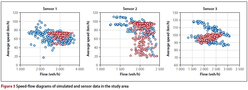
The simulation model was executed for validation purposes over a period of three hours and forty minutes, so as to include a 40-minute warm-up period, before starting to record vehicle counts over the subsequent three hours. The length of the warm-up period was determined according to the method outlined by Law and Kelton (2000), ensuring that a stable number of vehicles is present in the simulation model before data recording commences. This process was replicated thirty times with different seed values. The measured outputs at the sensor locations were then compared with the real-world values of the corresponding time period from 15:30 to 18:30. The results of this comparison are shown in Figure 5.

As may be seen in Figure 5, the simulated outputs, indicated in red, resemble the real-world measurements, indicated in blue. Note that neither the measured data nor the simulated output resembles the classical fundamental diagram. This may be due to the fact that only data from a specific, congestion-plagued period of time is shown. Based on the central limit theorem, one may assume that this data is normally distributed due to the large number of recorded values. Hypothesis tests were performed in order to ensure that the means of the simulated output and the real-world values do not differ statistically at a 5% level of significance.

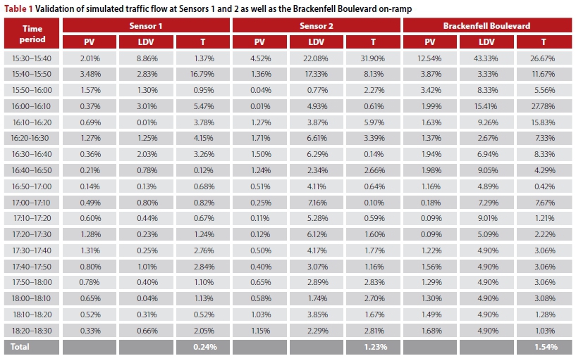
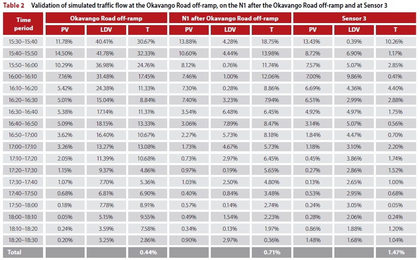
Furthermore, the average output results of these thirty replications were compared against the real-world measurements for all sensor and estimated locations from the first three Fridays of March 2017, and the absolute errors were recorded, as shown in Tables 1 and 2. As may be seen in the tables, the errors in respect of the flow of passenger vehicles, abbreviated in the tables as PV, never exceeded 2% during the simulated three-hour period. In terms of the light delivery vehicles, abbreviated in the tables as LDV, the maximum error during the three simulation hours rose to 4.90%. The reason for this is that the number of light delivery vehicles travelling through the system was significantly smaller than that of passenger vehicles, resulting in the phenomenon where even a small deviation in terms of the number of vehicles is reflected as a relatively large error when expressed as a percentage.

Finally, the largest error during the simulated three-hour period in terms of trucks travelling through the system, abbreviated in the tables as T, was 2.86%. As in the case of light delivery vehicles, however, relatively few trucks travelled through the system, and as a result a small error in terms of number is reflected as a relatively large error when expressed as a percentage. Due to the fact that the total error in respect of the number of vehicles that passed any of the six counting stations never exceeded 2%, the simulation model was deemed to be a sufficiently accurate representation of the underlying real-world system.

Model output data

The relative performances of the RL algorithms are measured according to the following performance measures (all measured in vehicle hours):

1. The total time spent in the system by all vehicles (TTS)

2. The total time spent in the system by vehicles entering the system from the N1 (TTSN1)

3. The total time spent in the system by vehicles entering the system from the R300 (TTSR300)

4. The total time spent in the system by vehicles entering the system from the Brackenfell Boulevard on-ramp (TTSBB), and

5. The total time spent in the system by vehicles entering the system from the Okavango Road on-ramp (TTSO).

The reason for breaking the TTS performance measure indicator down into the four further performance measures is that increases in the travel times of vehicles joining the highway from on-ramps at which RM is applied may not be captured sufficiently if only a single TTS performance measure were to be adopted. Now that the data inputs and outputs have been outlined, the focus of the discussion shifts to the calibration and validation of the simulation model.

 

NUMERICAL EXPERIMENTATION

The process followed throughout the numerical results evaluation is as follows. An Analysis of Variance (ANOVA) (Montgomery & Runger 2011) is performed in order to ascertain whether the simulation outputs from the different implementations differ statistically. Thereafter, Levene's Test (Schultz 1985) is performed in order to determine whether the variances of the output data sets are homogenous or not. If these variances are in fact homogenous, the Fischer LSD (Williams & Abdi 2010) post hoc test is employed in order to determine between which pairs of algorithmic output the differences occur. If, however, these variances are not homogenous, the Games-Howell (Games & Howell 1976) post hoc test is performed for this purpose.

Ramp metering

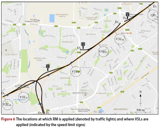
RM may be applied at all three on-ramps of the stretch of the N1 highway in Figure 4, namely the R300 on-ramp at O₂, the Brackenfell Boulevard on-ramp at O₃ and the Okavango Road on-ramp at O₄, as may be seen in Figure 6. As a benchmark for measuring the relative algorithmic performances in respect of RM, the ALINEA RM control strategy, which is often hailed as the benchmark RM control strategy (Rezaee et al 2013), is also implemented. In ALINEA, the metering rate is adjusted based on the difference in measured and target densities directly downstream of the on-ramp. In the ALINEA control law, a metering rate

 

 

 

measured in veh/h is assumed, where ρ* denotes the target density and P_ds(t) denotes the measured downstream density during time period t. Furthermore, PI-ALINEA is also implemented for additional comparative purposes. The metering rate to be applied following the PI-ALINEA control rule is

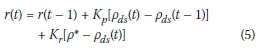
Finally the metering rate, taking into account the on-ramp queue consideration limit, may be calculated as

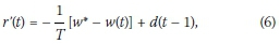
where T denotes the length of each control interval t, w(t) denotes the measured on-ramp queue length, w* denotes the maximum allowable on-ramp queue length, and d(t - 1) denotes the on-ramp demand during the previous time period t - 1. The final metering rate to be applied is then given by

for both ALINEA and PI-ALINEA. The red phase time to be applied in the microscopic traffic simulation model is then determined from the metering rate as

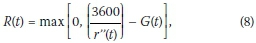
where G(t) denotes the fixed green phase duration applied at the on-ramp.

We consider five cases in which only RM is applied. In the first case, to serve as a benchmark, no control is applied, while in the second case, RM is enforced according to the modified ALINEA control law in (4). In the third case, the PI-ALINEA control law is adopted, while Q-Learning agents are employed to control the RM in the fourth case, and //NN-TD learning agents are employed for this purpose in the fifth case.

The R300 RM agent receives information on the downstream density p_dsat the section of highway directly downstream of the on-ramp where vehicles joining the highway from the on-ramp enter the highway traffic flow. The upstream density p_usis measured on the section of highway between the R300 off-ramp at D₁ and the R300 on-ramp at O₂, while the queue length w is the number of vehicles present in the R300 on-ramp queue.

The downstream density for the Brackenfell Boulevard RM agent is again measured at the section directly downstream of the on-ramp where the traffic flows from the on-ramp and the highway merge. The upstream density is measured on the section of highway between the R300 on-ramp at O₂ and the Brackenfell Boulevard on-ramp at O₃. Finally, the queue length is again the number of vehicles present in the on-ramp queue.

Similarly, for the Okavango Road RM agent, the downstream density is measured at the section where the on-ramp and highway traffic flows merge, while the upstream density is measured on the section of highway between the Okavango Road off-ramp at D2 and the Okavango Road on-ramp at O4. Finally, as was the case for both the other RM agents, the queue length is the number of vehicles present in the on-ramp queue.

An empirical parameter evaluation was performed to find the best-performing combination of on-ramps at which to employ RM in the case study area, as well as to determine the best-performing target densities for the RM agents at each on-ramp. In the case of ALINEA, PI-ALINEA and Q-Learning, having only one RM agent at the Okavango Road on-ramp, with a target density of 31.2 veh/km, 28.8 veh/km and 31.6 veh/km respectively, yielded the best performance. Furthermore, setting the value of Kr in (4) to 40 yielded the most favourable results for ALINEA. The controller parameters Kp and K_rin the PI-ALINEA implementation were set to 60 and 40 respectively, as these values yielded the best performance. For /NN-TD RM, having an RM agent at both the R300 on-ramp and the Okavango Road on-ramp, with target densities of 28.0 veh/km and 35.5 veh/km respectively, resulted in the best performance. Finally, the maximum allowable queue length was set to 50 vehicles at each of the on-ramps. A more detailed presentation of the parameter evaluations and algorithmic implementations may be found in Schmidt-Dumont (2018).

Summaries of the performances of the resulting algorithmic implementations are provided in Figure 7 and Table 3. The values of the aforementioned performance measures were calculated as the average values recorded after 30 independent simulation runs with varying seeds. For the purpose of comparison, however, the same 30 seed values were employed in each of the cases employing different RM agents.

 

 

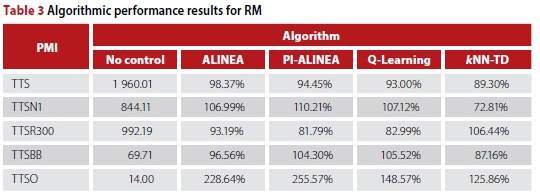
As may be seen in Table 3, all the RM implementations are able to improve on the no-control case in respect of the TTS.

Interestingly, /NN-TD RM is the only implementation that resulted in a reduction of the TTSN1. This may be explained by the fact that the highway flow is more protected as a result of RM at two of the three on-ramps, while vehicles experience congestion at the R300 on-ramp in all other implementations. As may have been expected, /NN-TD RM resulted in an increase in the TTSR300, as the flow of vehicles from the R300 is metered only in the /NN-TD RM implementation. The expected increases in the TTSO, due to RM at the Okavango Road on-ramp, are reflected by all RM implementations. Seeing that /NN-TD RM achieved the largest reduction in the TTS, it is considered to be the best-performing RM implementation.

Variable speed limits

VSL agents are implemented at each of the three interchanges in the case study area, as shown in Figure 6. As may be seen in the figure, two VSLs, namely VSLr and VSLr, are applied before the bottleneck at the R300 on-ramp. VSLr (which corresponds to VSL_usin Figure 3) is applied from the start of the simulated area at O₁ up to directly after the R300 off-ramp, which leads to D₁. Thereafter, VSLr (which corresponds to VSL_app in Figure 3) is applied until the R300 on-ramp. As there is only a single, relatively short section of highway between the R300 on-ramp and the Brackenfell Boulevard on-ramp, only a single VSL, namely VSL_b (which also corresponds to VSL_app in Figure 3), is applied on this section ahead of the expected bottleneck at the Brackenfell Boulevard on-ramp. This agent does, however, still receive information about the upstream density, measured on the section before the R300 on-ramp. After the Brackenfell Boulevard on-ramp, the first of the VSLs corresponding to the agent located at the Okavango Road on-ramp, namely VSLq (which again corresponds to VSL_us in Figure 3), is applied. This speed limit is enforced until directly after the Okavango Road off-ramp which leads to D₂. After the off-ramp at the Okavango Road interchange, VSLq (which corresponds to VSL_app in Figure 3) is applied up to the section directly after the Okavango Road on-ramp, at which point the normal speed limit of 120 km/h is restored.

Similarly to the RM implementations, a feedback controller was implemented as a performance benchmark for the RL implementations. The chosen feedback controller is the so-called mainline traffic flow controller (MTFC) by Müller et al (2015). The control structure of this controller is similar to that of ALINEA, as a VSL metering rate

is assumed, where Kj denotes the controller parameter, and ρ* and ρ_dsagain denote the target and measured downstream density, respectively. The VSL to be applied at the section VSL_appin Figure 3 is then given by

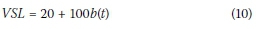
rounded to the nearest 10 km/h, resulting in speed limits

VSL ε {20, 30, 40, 50, 60, 70, 80, 90, 100, 110, 120}.

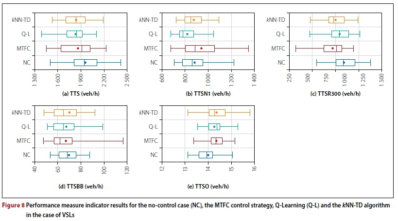
As for the RM implementations, a parameter evaluation was performed for VSLs in order to determine the best-performing combination of VSL agents in the case study area, as well as the best-performing Kj-value in (9) and δ-value in (3) for updating VSL_r1and VSLq respectively. This parameter evaluation revealed that the best performance is achieved with an MTFC controller at the Okavango Road interchange with a Kj-value set to 0.005 and target density set to 37 veh/km. The best performance for Q-Learning was achieved having a VSL agent at the R300 interchange with δ = 10, and a VSL agent at the Brackenfell Boulevard interchange. For / NN-TD VSL the best performance is achieved for a VSL agent with δ = 20 at the R300 interchange, and a VSL agent at the Okavango Road interchange with δ = 10. Summaries of the resulting algorithmic performances are provided in Figure 8 and Table 4.

 

 

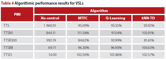
As may be seen in the Table 4, all three VSL implementations were able to achieve reductions in the TTS. In the case of the RL implementations, these reductions are a result of reduced travel times for vehicles travelling along the N1 and entering the N1 from the R300 on-ramp. This may have been expected as these are the vehicles that spend the longest time on the N1, where VSLs have the largest effect. The reduction in the TTSR300 furthermore suggests that effective applications of VSLs may improve the process whereby vehicles from the R300 join the N1 highway. Finally, the reduced variances, as may be seen in Figure 8(b), suggest that there may be successful homogenisation of traffic flow on the N1 due to VSLs. The improvements in respect of the MTFC controller were achieved mainly by those vehicles joining the N1 from the R300, as these vehicles experienced the benefit of VSLs at the Okavango Road interchange, while the effectiveness for vehicles travelling along the N1 only was limited, due to these vehicles still experiencing congestion at the R300 on-ramp merge.

MARL for RM and VSLs

As a benchmark for the MARL implementations, the integrated feedback controller of Carlson et al (2014) is implemented. RM occurs according to the PI-ALINEA control law with the addition of a queue limit as in (5), while the MTFC controller of Müller et al (2015) is employed for the control of VSLs.

Due to the finding that both PI-ALINEA and MTFC were most effective at the Okavango Road interchange, only one integrated controller is implemented at this interchange.

Due to the fact that the //NN-TD learning algorithm achieved the largest reductions in the TTS in both the single agent implementations, only the //NN-TD algorithm is implemented in the three MARL approaches. For both the RM and VSL implementations, the best results were achieved by having two RM or VSL //NN-TD RL agents in the case study area. The first of these is at the R300 interchange, while the second is at the Okavango Road interchange. As a result, only these two locations are considered for the MARL implementations. The first MARL implementation corresponds to the R300 interchange and consists of the ramp meter placed at the R300 on-ramp, denoted by O₂, and the speed limits VSLr and VSLr . The target density of the agents in this MARL implementation is set to 28 veh/km, which was determined to be the best-performing target density in the RM parameter evaluation at the R300 on-ramp. VSLr is updated with δ = 20, which was found to yield the best results in the VSL parameter evaluation conducted for VSLs at the R300 interchange.

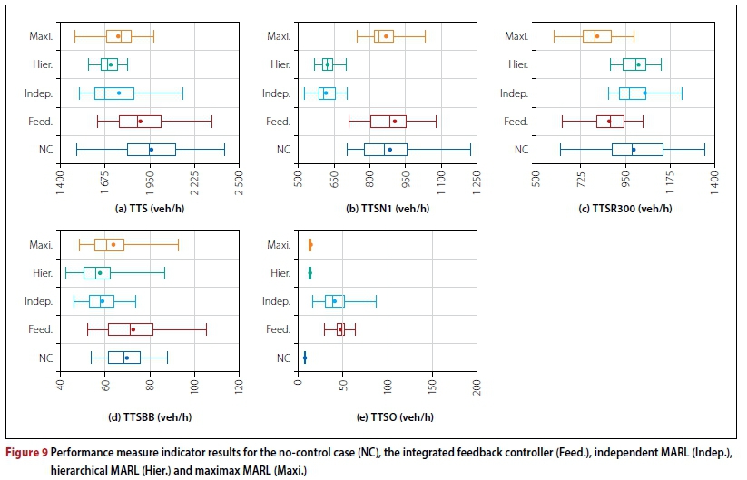
The second MARL implementation controls the ramp meter placed at the Okavango Road on-ramp, denoted by O₄, and the speed limits VSLq and VSLq . The target density of the agents in the second MARL implementation is set to 35.5 veh/km, which was determined to be the best-performing target density in the RM parameter evaluation. Finally, VSLq is updated with δ = 10, which was found to yield the best performance in the VSL parameter evaluation. Summaries of the results achieved by the MARL implementations are provided in Figure 9 and Table 5.

 

 

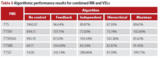
As may be seen in Table 5, employing MARL in order to solve the RM and VSL problems simultaneously may lead to further reductions in respect of the TTS, when compared with the singleagent implementations. Furthermore, the combination of RM and VSLs may lead to improved homogenisation of traffic flow, as may be deduced from the smaller variances of the box plots corresponding to the MARL approaches in Figure 9. Finally, the MARL implementations were again able to outperform the integrated feedback controller, providing an illustration of the effectiveness of the MARL approach when compared with the current uncontrolled situation, as well as with the state-of-the-art feedback controller.

 

CONCLUSIONS

The results obtained from the RM implementations demonstrate that RM may effectively be employed to reduce the total travel time spent by vehicles in the system by up to 10.70% when compared with the no-control case in the context of the case study. Furthermore, the RL approaches to RM outperformed ALINEA and PI-ALINEA, which achieved reductions of only 1.63% and 5.55% respectively. Furthermore, / NN-TD learning was able to find the best trade-off between balancing the length of the on-ramp queue and protecting the highway flow. / NN-TD RM was also the only implementation able to reduce the TTS when an RM agent is present at the R300 on-ramp.

Although they were not quite as effective as RM in reducing the TTS, the VSL implementations resulted in significant reductions in the TTS of 6.45⁰% and 6.08% by Q-Learning and / NN-TD VSL respectively, while the MTFC controller achieved a reduction of 4.91% when compared with the no-control case. One reason for this may be homogenisation of traffic flow, as the traffic flow becomes more stable at lower speeds, while the results suggest that the process by which vehicles join the N1 from the R300 on-ramp also occurs more smoothly if VSLs are employed in an effective manner.

Finally, employing a MARL approach to solving the RM and VSL problems simultaneously has shown that further reductions in the TTS are possible when these control measures are employed together, as independent MARL, hierarchical MARL and maximax MARL achieved reductions in the TTS of 10.13%, 12.70% and 10.39% respectively over the no-control case. The integrated feedback controller, on the other hand, was only capable of achieving an improvement of 3.36%. Notably, the hierarchical MARL and maximax MARL approaches were able to find the most effective balance between managing the on-ramp queue at the Okavango Road on-ramp and protecting the highway traffic flow, as both of these implementations did not result in statistically significant increases in respect of the TTSO. Based on these results, we believe there is a strong case to be made in respect of considering the adoption of hierarchical MARL for RM and VSLs on South African highways within urban areas, as significant reductions in the travel times experienced by motorists may be expected.

 

ACKNOWLEDGEMENTS

The authors would like to thank Mrs Megan Bruwer from the Stellenbosch Smart Mobility Laboratory within the Department of Civil Engineering at Stellenbosch University for her assistance in obtaining the data required for this study.

 

LIST OF ACRONYMS

ALINEA - Asservissement Lineaire d'entrée Autorotiere

ANOVA - Analysis of Variance

k/NN-TD - /-Nearest Neighbour Temporal Difference

LDV - Light Delivery Vehicle

MARL - Multi-agent Reinforcement Learning

MPC - Model Predictive Control

MTFC - Mainline Traffic Flow Control

PV - Passenger Vehicle

RM - Ramp Metering

R-MART - R-Markov Average Reward Technique

RL - Reinforcement Learning

TTS - Total Time Spent in the System by all Vehicles

TTSN1 - Total Time Spent in the System by Vehicles entering from the N1

TTSR300 - Total Time Spent in the System by Vehicles entering from the R300

TTSBB - Total Time Spent in the System by Vehicles entering from Brackenfell Boulevard

TTSO - Total Time Spent in the System by Vehicles entering from Okavango Road

VSL - Variable Speed Limit

 

REFERENCES

Alessandri, A, Di Febbraro, A, Ferrara, A & Punta, E 1998. Optimal control of freeways via speed signalling and ramp metering. Control Engineering Practice, 6(6): 771-780.         [ Links ]

Alessandri, A, Di Febbraro, A, Ferrara, A & Punta, E 1999. Nonlinear optimization for freeway control using variable-speed signalling. IEEE Transactions on Vehicular Technology, 48(6): 2042-2052.         [ Links ]

Amirjamshidi, G & Roorda, M 2017. Multi-objective calibration of traffic microsimulation models. Transportation Letters, 9(1): 1-9.         [ Links ]

AnyLogic 2017. Multimethod simulation software. Available at: http://www.anylogic.com [accessed on 31 January 2017].         [ Links ]

Busoniu, L, Babuska, R & De Schutter, B 2008. A comprehensive survey of multi-agent reiforcement learning. IEEE Transactions on Systems Managament and Cybernetics. Part C: Applications and Reviews, 38(2): 156-172.         [ Links ]

Carlson, R C, Papamichail, I, Papageorgiou, M & Messmer, A 2010. Optimal motorway traffic flow control involving variable speed limits and ramp metering. Transportation Science, 44(2): 238-253.         [ Links ]

Carlson, R C, Papamichail, I & Papageorgiou, M 2011. Local feedback-based mainstream traffic flow control on motorways using variable speed limits. IEEE Transactions on Intelligent Transportation Systems, 12(4): 1261-1276.         [ Links ]

Carlson, R C, Ioannis, P & Papageorgiou, M 2014. Integrated feedback ramp metering and mainstream traffic flow control on motorways using variable speed limits. Transportation Research. Part C: Emerging Technologies, 46: 209-221.         [ Links ]

Committee of Transport Officials (COTO) 2013. South African standard automatic traffic data collection format. Pretoria: South African National Roads Agency Limited.         [ Links ]

Davarjenad, M, Hegyi, A, Vrancken, J & Van den Berg, J 2011. Motorway ramp-metering control with queueing consideration using Q-learning. Proceedings, 14th International IEEE Conference on Intelligent Transportation Systems, 5-7 October 2011, Washington, DC. pp 1652-1658.         [ Links ]

El Tantawy, S, Abduhai, B & Abdelgawad, H 2013. Multiagent reinforcement learning for an integrated network of adaptive traffic signal controllers (MARLIN-ATSC): Methodology and large-scale application in downtown Toronto. IEEE Transactions on Intelligent Transportation Systems, 14(3): 1140-1150.         [ Links ]

Games, P A & Howell, J F 1976. Pairwise multiple comparison procedures with unequal n's and/ or variances: A Monte Carlo study. Journal of Educational Statistics, 1(2): 113-125.         [ Links ]

Hegyi, A, De Schutter, B & Hellendoorn, H 2005. Model predictive control for optimal coordination of ramp metering and variable speed limits. Transportation Research. Part C: Emerging Technologies, 35(2): 185-209.         [ Links ]

Law, A & Kelton, W 2000. Simulation Modelling and Analysis, 3rd ed. Boston, MA: McGraw-Hill.         [ Links ]

Martin, J, De Lope, J & Maravall, D 2011. Robust high-performance reinforcement learning through weighted k-nearest neighbours. Neurocomputing, 74(8): 1251-1259.         [ Links ]

Montgomery, D C & Runger, G C 2011. Applied Statistics and Probability for Engineers, 5th edition. New York: Wiley.         [ Links ]

Müller, E R, Carlson, R C, Kraus, W & Papageorgiou, M 2015. Microsimulation analysis of practical aspects of traffic control with variable speed limits. IEEE Transactions on Intelligent Transportation Systems, 16(1): 512-523.         [ Links ]

Nair, R, Varakantham, P, Tambe, M & Yokoo, M 2005. Networked distributed POMPDs: A synthesis of distributed constraint optimization and POMPDs. Proceedings, 20th National Conference on Artificial Intelligence, 9-13 July 2005, Pittsburgh, PA.         [ Links ]

Noland, R 2001. Relationships between highway capacity and induced vehicle travel. Transportation Research. Part A: Policy and Practice, 1(35): 47-72.         [ Links ]

Papageorgiou, M & Kotsialos, A 2000. Freeway ramp metering: An overview. IEEE Transactions on Intelligent Transportation Systems, 3(4): 271-281.         [ Links ]

Papageorgiou, M, Hadj-Salem, H & Blosseville, J-M 1991. ALINEA: A local feedback control law for on-ramp metering. Transportation Research Record, 1320: 90-98.         [ Links ]

Papamichail, I, Kotsialos, A, Margonis, I & Papageorgiou, M 2010. Coordinated ramp metering for freeway networks: A model predictive hierarchical control approach. Transportation Research. Part C: Emerging Technologies, 18(3): 311-331.         [ Links ]

Rezaee, K, Abduhai, B & Abdelgawad, H 2013. Self-learning adaptive ramp metering: Analysis of design parameters on a test case in Toronto, Canada. Transportation Research Record, 2396(1): 10-18.         [ Links ]

SANRAL (South African National Roads Agency Limited) 2009. Gauteng Freeway Improvement Project. Available at: http://www:nra:co:za/live/content:php?SessionID=ba5532d579e74187850e66750126832a&ItemID=260 [accessed on 29 August 2017].         [ Links ]

Schmidt-Dumont, T 2018. Reinforcement learningfor the control of traffic flow on highways. PhD thesis. Stellenbosch University.         [ Links ]

Schranck, D, Eisele, B & Lomax, T 2012. Til's 2012 urban mobility report. College Station, TX: Texas A&M Transportation Institute.         [ Links ]

Schultz, B B 1985. Levene's test for relative variation. Systematic Biology, 34(4): 449-456.         [ Links ]

Smaragdis, E & Papageorgiou, M 2003. Series of new local ramp metering strategies. Transportation Research Record, 1856: 74-86.         [ Links ]

Smulders, S 1990. Control of freeway traffic flow by variable speed signs. Transportation Research. Part B: Methodological, 24(2): 111-132.         [ Links ]

Sutton, R S & Barto, A G 1998. Reinforcement Learning: An Introduction. Cambridge, MA: MIT Press.         [ Links ]

Szepesvari, C 2010. Algorithms for reinforcement learning. Synthesis Lectures on Artificial Intelligence and Machine Learning, 4(1): 1-103.         [ Links ]

TomTom 2017. TomTom traffic index: Measuring congestion worldwide. Available at: https://www.tomtom.com/en_gb/trafficindex [accessed on 7 November 2017].         [ Links ]

Walraven, E, Spaan, M & Bakker, B 2016. Traffic flow optimization: A reinforcement learning approach. Engineering Applications of Artificial Intelligence, 52(1): 203-212.         [ Links ]

Wang, Y, Kosmatopolous, E B, Papgeorgiou, M & Papamichail, I 2014. Local ramp metering in the presence of a distant downstream bottleneck: Theoretical analysis and simulation study. IEEE Transactions on Intelligent Transportation Systems, 15(5): 2024-2039.         [ Links ]

Watkins, C & Dayan, P 1992. Q-learning. Machine Learning, 8(3-4): 279-292.         [ Links ]

Wattleworth, J 1967. Peak period analysis and control of a freeway system/with discussion. Highway Research Record, 157(1): 1-21.         [ Links ]

Wavetronix 2017. SmartSensor HD: Arterial and freeway. Available at: https://www:wavetronix:com/en/products/3-smartsensor-hd [accessed on 6 June 2017].         [ Links ]

Williams, L H & Abdi, H 2010. Fisher's least significant difference (LSD) test. In: Salkind, N. (Ed.), Encyclopedia of Research Design, Thousand Oaks, CA, 1-6.         [ Links ]

Zhu, F & Ukkusuri, S 2014. Accounting for dynamic speed limit control in a stochastic traffic environment: A reinforcement learning approach. Transportation Research. Part C: Emerging Technologies, 41(1): 30-47.         [ Links ]

 

 

Correspondence:
DR THORSTEN SCHMIDT-DUMONT
Stellenbosch Unit for Operations Research in Engineering
Department of Industrial Engineering
Stellenbosch University
Private Bag X1
Matieland 7602
South Africa
T: +27 21 808 4233
E: thorstens@sun.ac.za

PROF JAN H VAN VUUREN
Stellenbosch Unit for Operations Research in Engineering
Department of Industrial Engineering
Stellenbosch University
Private Bag X1
Matieland 7602
South Africa
T: +27 21 808 4244
E: vuuren@sun.ac.za

 

 

 

DR THORSTEN SCHMIDT-DUMONT was born in Swakopmund, Namibia, in 1993. He received the B.Eng and PhD (Industrial Engineering) degrees in 2015 and 2018 respectively from Stellenbosch University, and has since taken up a position as post-doctoral research fellow within the Department of Industrial Engineering at Stellenbosch University. He is the author of one journal publication and one paper published in peer-reviewed conference proceedings, and has attended and presented his work at local and international conferences. His research interests include systems optimisation, machine learning and the application thereof to real-world systems.

 

 

PROF JAN H VAN VUUREN (Pr Sci Nat) was born in Durban, South Africa, in 1969. He obtained a Master's in applied mathematics from Stellenbosch University in 1992 and a doctorate in mathematics from the University of Oxford, United Kingdom, in 1995. Since 1996 he has been a member of staff at Stellenbosch University where he is currently professor of operations research within the Department of Industrial Engineering. He is the author of 97 journal publications and 32 peer-reviewed conference proceeding papers. His research interests include combinatorial optimisation and decision-support systems.