TECHNICAL PAPER

 

Catchment response time and design rainfall: the key input parameters for design flood estimation in ungauged catchments

 

 

O J Gericke

Correspondence

 

 

---

ABSTRACT

Catchment response time and design rainfall are regarded as fundamental input to all design flood estimation methods in ungauged catchments, while errors in estimated catchment response time and design rainfall directly impact on estimated peak discharges. This paper presents the independent testing and comparison of the latest catchment response time and design rainfall estimation methodologies with current well-known and simplified methodologies used in South Africa to ultimately highlight the impact thereof on design flood estimation. The results confirmed that catchment response time, design rainfall, and to some lesser extent runoff coefficients, are the key input parameters for design flood estimation in ungauged catchments and have a significant impact on the design of hydraulic structures. It is recommended that the current well-known and simplified catchment response time (USBR T_Cequation) and design rainfall (modified Hershfield/TR102 DDF approach) estimation methodologies should be replaced with the empirical G&S T_Cequations and the RLMA&SI DDF approach when deterministic design floods are estimated in ungauged catchments in South Africa.

Keywords: catchment response time, design rainfall, design flood estimation, ungauged catchments

---

 

 

INTRODUCTION

Design flood estimation is necessary for the planning, design and operation of hydraulic structures, e.g. culverts, bridges and/or spillways at a particular site in a specific region (Pegram & Parak 2004). In South Africa, three basic approaches to design flood estimation are available, namely the probabilistic, deterministic and empirical methods (Parak & Pegram 2006; Smithers 2012; Van der Spuy & Rademeyer 2016). In gauged catchments, despite uncertainties and errors in measurement, observed peak discharges are regarded as the best estimate of the true peak discharge (Gericke & Smithers 2016b). In terms of design flood estimation in gauged catchments, probabilistic methods that are adequate in both length and quality of data are normally used to conduct a frequency analysis of observed flood peak data from a flow-gauging site (Smithers 2012). In ungauged catchments, practitioners are required to estimate design floods using either deterministic and/or empirical methods, although regional probabilistic methods or continuous simulation models could also be used to transfer design values from gauged to ungauged sites.

Single-event deterministic design flood estimation methods are the most commonly used by practitioners in ungauged catchments (Van Vuuren et al 2012). In the application of these single-event deterministic methods, all complex, heterogeneous catchment processes are lumped into a single process to enable the estimation of the expected output (design flood) from causative input (design rainfall) in a simple and robust manner (Gericke & Du Plessis 2013). Design rainfall comprises a depth and duration (directly proportional to the catchment response time) associated with a given annual exceedance probability (AEP) or return period (T).

The catchment response time is normally expressed as a single time parameter, e.g. time of concentration (T_c), lag time (T_L) and/or time to peak (T_p). In other words, estimates of peak discharge are based on a single representative catchment response time parameter (e.g. Tp, T_cand/ or T_L), while the catchment is at an 'average condition' and the hazard or risk associated with a specific event is reflected by the joint-probability of the 1:T-year design rainfall and 1:T-year design flood events (Rahman et al 2002; SANRAL 2013). This assumption considers the probabilistic nature of rainfall, but the probabilistic behaviour of other inputs and parameters is ignored. Taking into consideration the vast complexity and spatial and temporal variability of catchment processes and their driving forces, as well as the probable significant bias introduced by ignoring the joint-probability of rainfall and runoff, it is not surprising that only relatively simple deterministic methods representing the real world processes are recognised and used in design flood practice (Smithers 2012).

Catchment response time and design rainfall are therefore regarded as fundamental input to all design flood estimation methods in ungauged catchments, while errors in estimated catchment response time and design rainfall will directly impact on estimated peak discharges. Bondelid et al (1982) indicated that as much as 75% of the total error in design peak discharge estimates in ungauged catchments could be ascribed to errors in the estimation of catchment response time parameters. Grimaldi et al (2012) highlighted that estimates of catchment response time, using different equations, may differ from each other by up to 500%. Gericke and Smithers (2014) also showed that the underestimation of time parameters by 80% or more could result in slightly lower design rainfall depths, although of much higher intensities, hence ultimately resulting in the overestimation of design peak discharges of up to 200%.

Empirical time parameter estimation methods are widely used in South Africa, with only the T_Lmethods proposed by Pullen (1969) and Schmidt and Schulze (1984) being developed locally. In terms of T_cestimation, the empirical Kerby (1959) and United States Bureau of Reclamation (USBR 1973) equations are recommended for general use in South Africa for overland and channel flow conditions respectively (SANRAL 2013). However, both these equations were developed and calibrated in the United States of America (USA) for catchment areas less than 4 ha and 45 ha respectively (McCuen et al 1984). Gericke and Smithers (2014; 2016a; 2016b) highlighted the inherent limitations and inconsistencies introduced when these T_cequations, which are currently recommended for general practice in South Africa, are applied outside their bounds, both in terms of areal extent and their original regions of development, without using any local correction factors. In a recent study, Gericke and Smithers (2016b; 2017) used observed catchment response time parameters to derive new empirical time parameter equations for medium to large catchments in South Africa. These derived catchment-specific/regional empirical time parameter equations (referred to as G&S T_cequation in this paper) resulted in improved peak discharge estimates when compared to the USBR T_cequation in 60 of the 74 catchments considered.

In terms of design rainfall, Gericke and Du Plessis (2011) evaluated five depth-duration-frequency (DDF) approaches commonly used in South Africa to estimate design rainfall depths. The DDF approaches that were evaluated included those based on: (i) Log-Extreme Value Type I (LEV1) distributions (Midgley & Pitman 1978), (ii) Technical Report 102 (TR102) daily design rainfall information (Adamson 1981), (iii) Regional Linear Moment Algorithm South African Weather Services (RLMA-SAWS) n-day design point rainfall information (Smithers & Schulze 2000b), (iv) modified Hershfield equation (Alexander 2001), and (v) Regional Linear Moment Algorithm and Scale Invariance (RLMA&SI) approach (Smithers & Schulze 2003; 2004). It was recommended that the M&P/LEV1 and modified Hershfield DDF relationships should be seen as conservative estimates, and their use should be limited to small (T_c < 6 hours) and medium-sized (6 < T_c< 24 hours) catchments, while the RMLA&SI approach should be regarded as the standard DDF relationship for all catchment response times and catchment sizes under consideration.

Potential future improvements in peak discharge estimation using event-based design flood estimation methods will not be realised if practitioners continue to use inappropriate time parameter and design rainfall estimation methods. Not only will the accuracy of design flood estimation methods be limited, but it will also have an indirect impact on hydraulic designs, i.e. underestimated time parameter values and higher design rainfall intensities will result in overdesigned hydraulic structures, and the overestimation of time parameters associated with lower design rainfall intensities will result in underdesigns.

The study objectives and assumptions are discussed in the next section, followed by a summary of the study area. Thereafter, the methodologies involved in meeting the objectives are detailed, followed by the results, discussion and conclusions.

 

STUDY OBJECTIVES AND ASSUMPTIONS

The overall objective of this study is to independently test and compare the latest catchment response time and design rainfall estimation methodologies with current well-known and simplified methodologies used in South Africa to ultimately highlight the impact thereof on design flood estimation. The specific objectives are to: (i) conduct at-site probabilistic flood frequency analyses in gauged catchments, (ii) compare and evaluate the combined use of the recommended USBR T_cequation (USBR 1973) and modified Hershfield DDF approach and/or TR102 design rainfall information (Adamson 1981) to the combined use of the empirical G&S T_cequations (Gericke & Smithers 2016b; 2017) and the RLMA&SI DDF approach (Smithers & Schulze 2003; 2004), (iii) translate the time parameter and design rainfall estimation results to design peak discharges using an appropriate single-event deterministic design flood estimation method, (iv) verify and test the consistency, robustness and accuracy of the deterministic design estimates (Q_t) by comparing these design estimates with the at-site probabilistic flood frequency analyses (Q_p), and (v) highlight the impact of these over- or underestimations on prospective hydraulic designs, while attempting to identify the influence of possible source(s) that might contribute to the differences in the estimation results.

The Standard Design Flood (SDF) method (Alexander 2002; Gericke & Du Plessis 2012; SANRAL 2013) was selected as the most suitable single-event deterministic method to estimate the design peak discharges, since it is: (i) a regionally calibrated version of the Rational method and is not subject to user-biasedness in terms of the selection of site-specific runoff coefficients, (ii) deterministic-probabilistic in nature, and (iii) applicable to catchment areas up to 40 000 km², which coincide with the catchment area ranges considered in this study, e.g. 28 km2 to 31 283 km².

The use of the SDF method is further justified given that the primary focus of this paper is on the impact of catchment response time and design rainfall estimates on peak discharge, and not on the design flood estimation method itself.

This study is based on the following assumptions:

■ The conceptual T_cequals Tp. The conceptual T_cis normally defined as the time required for the entire catchment to contribute runoff at the catchment outlet, while T_pis defined as the time interval between the start of effective rainfall and the peak discharge of a single-peaked hydrograph (McCuen et al 1984; McCuen 2005; USDA NRCS 2010; SANRAL 2013). However, this definition of T_pis also regarded as the conceptual definition of T_C(McCuen et al 1984; Seybert 2006) and Gericke and Smithers (2014) also showed that T_c~ T_p.

■ Channel flow dominates the catchment response time in medium to large catchments and is representative of the total travel time; hence, the current common practice to divide the principal flow path into segments of overland flow and channel flow to estimate the total travel time was not applied.

■ Practitioners tend to use only well-known and simplified DDF relationships to estimate design rainfall depths, irrespective of whether numerical or graphical methods are used. This is probably due to the probabilistic rainfall frequency analyses that need to be conducted to convert observed daily point rainfall to a design rainfall depth associated with the catchment response time, as well as the uncertainty of the relative applicability thereof and whether the rainfall magnitude-frequency relationships will be satisfactorily accommodated in these alternatives.

 

STUDY AREA

South Africa is located on the southernmost tip of Africa and is demarcated into 22 primary drainage regions (A to X) as shown in Figure 1. These primary drainage regions are further delineated into 148 secondary drainage regions, i.e. A1, A2 to X4 (Midgley et al 1994). The 48 gauged catchments in this study are located in 23 of these secondary drainage regions comprising SDF basins 1-3, 9, 17, 18 and 23-26, which are located in four distinctive climatological regions of South Africa, i.e. the Northern Region (NR), Central Region (CR), Southern Winter Coastal Region (SWCR) and Eastern Summer Coastal Region (ESCR) (Gericke and Smithers 2016b; 2017). The four climatological regions are representative of the broad variations in climate (e.g. mean annual precipitation (MAP), rainfall type, distribution and rainfall seasonality), catchment geomorphology, channel geomorphology, geographical location, and altitude above mean sea level found in South Africa.

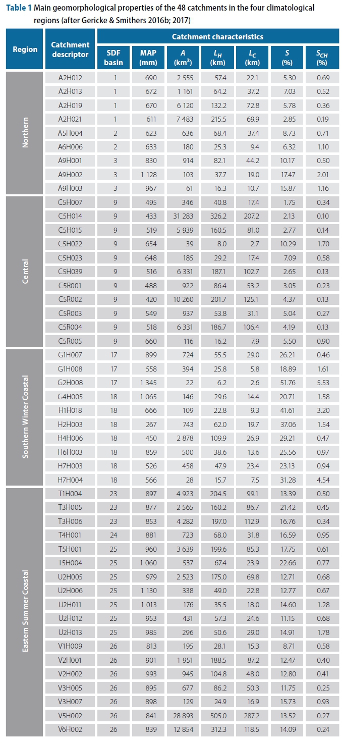
The catchment areas range between 28 km² and 31 283 km² and are regarded as 'gauged', since Department of Water and Sanitation (DWS) flow-gauging stations are located at the outlet of each catchment. Table 1 contains a summary of the SDF basin numbers and main geomorphological catchment properties, e.g. MAP, catchment area (A), hydraulic length (L_H), centroid distance (L_c), average catchment slope (S) and main river slope (S_ch), for each catchment under consideration.

The influences of each variable or parameter listed in Table 1 are highlighted, where applicable, in the subsequent sections. The DWS station numbers are also used as catchment descriptors for easy reference in all the subsequent tables and figures.

 

METHODOLOGY

This section provides the detailed methodology applied in each of the 48 gauged catchments. The following procedures were performed: (i) at-site probabilistic flood frequency analyses, (ii) estimation of catchment response time, (iii) estimation of design rainfall, and (iv) estimation of deterministic design floods.

At-site probabilistic flood frequency analyses

Seventy-nine gauged catchments were initially considered for possible inclusion in this study, but only 48 catchments met the following screening criteria: (i) streamflow record lengths (N) > 25 years, and (ii) the use of standard DWS discharge rating tables within the maximum rated flood level (H). However, in some cases where the observed flood levels exceeded H, the extrapolation of the rating curves up to or beyond bankfull flow conditions were considered. The high flow extensions above bankfull flow conditions were only considered in cases where the existing DWS discharge rating table included floodplain flow on the full width of the floodplain. In essence, the individual stage extrapolations H_e), whether for bankfull or above bankfull flow conditions, were limited to a maximum of 30%, i.e. H_E< 1.3 H. Only 40 events (1.5%) of the total of 2 665 annual maximum series (AMS) events analysed were subjected to such H_eextrapolations, i.e. 17 events with H_e< 1.1 H, 7 events with 1.1 H < H_E< 1.15 H, 8 events with 1.15 H < H_E< 1.20 H, and 8 events with 1.20 H < H_E< 1.30 H.

At-site probabilistic flood frequency analysis of the AMS was conducted at the 48 flow-gauging stations to summarise the observed flood peaks, estimate parameters and select appropriate theoretical probability distributions. The observed flood peaks were summarised by ranking the AMS in a descending order of magnitude, and the Cunnane plotting position (Equation 1; SANRAL 2013) was used to assign AEP or T values to the plotted values.

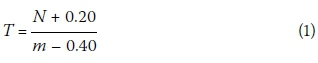
Where:

T = return period (years)

m = number, in descending order, of the ranked AMS events

N = record length (years)

The Method of Moments (MM) and Linear Moments (LM) were used to estimate parameters to ultimately enable the fitting of theoretical probability distributions to the AMS values. Statistical properties (e.g. mean, standard deviation, skewness and coefficient of variation) of each AMS (normal and log₁₀-transformed) and visual inspection of the plotted values were used to select the most suitable theoretical probability distribution in each catchment. The Log-Normal (LN) distribution was only considered where the logarithms of the AMS have a near symmetrical distribution or where the skewness coefficients were close to zero. In all other asymmetrical data sets, the Log-Pearson Type 3 (LP3), General Extreme Value (GEV) and/or General Logistic (GLO) distributions were considered.

Estimation of catchment response time

The catchment response time was estimated using both the USBR (1973) equation (Equation 2), which is currently widely used in South Africa, and the new regional G&S equation (Equation 3) derived by Gericke and Smithers (2016b; 2017).

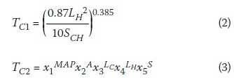
Where:

T_c1,2 = time of concentration (hours)

A = catchment area (km²)

L_c = centroid distance (km)

L_H = hydraulic length (km)

MAP = mean annual precipitation (mm)

S = average catchment slope (%)

S_ch = average main river slope (%)

X₁to X₅ = regional calibration coefficients as listed in Table 2

Estimation of design rainfall

The design rainfall information was estimated using two different DDF approaches. The first set of design point rainfall depths and intensities was based on the modified Hershfield equation (Equation 4; Alexander 2001) and/or TR102 design rainfall information with the associated critical storm durations (T_C1) estimated using Equation 2.

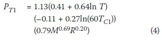
Where:

p_T1 = design point rainfall depth (mm) M = 2-year mean of the annual daily maxima rainfall (mm)

R = average number of days per year on which thunder was heard (days/ year)

T = return period (years)

T_c1 = time of concentration estimated using Equation 2 (hours)

Equation 4 is only applicable to T_cvalues less than six hours. For T_cvalues exceeding six hours and less than 24 hours, linear interpolation was applied between Equation 4 and the one-day design rainfall depths from TR102. In cases where T_cexceeded 24 hours, linear interpolation between the n-day design rainfall depth values was used (SANRAL 2013).

The second set of design point rainfall depths and intensities was based on the RLMA&SI approach (p_T2) and associated critical storm durations (T_c2) estimated using Equation 3. The RLMA&SI approach is automated and is included in the software program, Design Rainfall Estimation in South Africa (Smithers & Schulze 2003; 2004), which facilitates the estimation of design rainfall depths at a spatial resolution of 1-arc minute, for any location in South Africa, for durations ranging from 5 minutes to 7 days, and for return periods of 2 to 200 years. The RLMA&SI gridded design point and average catchment design point rainfall values were estimated by making use of the following steps in the ArcGIS™ environment:

■ Step 1: The average catchment design point rainfall representative of the average meteorological conditions in each catchment was estimated by applying the Thiessen polygon method (Wilson 1990) to all the daily design rainfall stations (from the RLMA-SAWS database) within the catchment boundary. Both the MAP and average design point rainfall depths for storm durations of 1 to 7 days were estimated.

■ Step 2: A single rainfall station located approximately at the geographical centre of each catchment, and which is representative of the average meteorological conditions as estimated in Step 1, was then selected from those rainfall stations used in Step 1 as the base station to estimate the RLMA&SI gridded design point rainfall values.

■ Step 3: With the single rainfall station as selected in Step 2, the appropriate critical storm durations (e.g. 5 minutes to 7 days), return periods (e.g. 2 to 200 years) and block size (e.g. spatial resolution of 1' χ 1' grid points), were selected. The block size was specified in such a way that the whole extent of each catchment under consideration is covered with grid points. The latter block of grid points was then extracted using the clip tool available from the Extract toolset contained in the Analysis Tools toolbox to include only the grid points within the boundary of each catchment.

■ Step 4: Lastly, the gridded point values for the catchment-specific critical storm durations (T_aand T_c2) and return periods under consideration were converted to an average catchment value using the arithmetic mean and linear interpolation, respectively.

Areal reduction factors (ARFs) were estimated using Equation 5 (Alexander 2001; SANRAL 2013) in order to convert the average design point rainfall depths or intensities to average areal design rainfall depths or intensities.

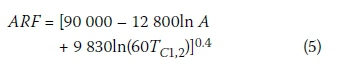
Where:

ARF = areal reduction factor (%)

A = catchment area (km²)

T_{c1, 2} = time of concentration estimated using either Equations 2 or 3 (hours)

Estimation of deterministic design floods

The time parameter and design rainfall results based on the combined use of Equations 2, 4 and 5, and Equations 3, 5 and the RLMA&SI approach, served as input to the SDF method (Equation 6; Alexander 2002) to ultimately estimate the deterministic design floods.

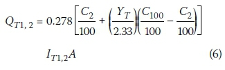
Where:

Q_t1= design peak discharge (m³/s) estimated using the standard SDF method

Q_T2= design peak discharge (m³/s) estimated using the new SDF procedure

A = catchment area (km²)

C₂= 2-year return period runoff coefficient

C₁₀₀= 100-year return period runoff coefficient

I_t1= average areal design rainfall intensity (mm/h) estimated using Equations 2, 4 and Equation 5 I_T2 = average areal design rainfall intensity (mm/h) estimated using Equations 3, 5 and the RLMA&SI approach Y_t= return period factor

 

RESULTS AND DISCUSSION

The results from the application of the above methodology in the 48 catchments are presented in this section.

At-site probabilistic flood frequency analyses

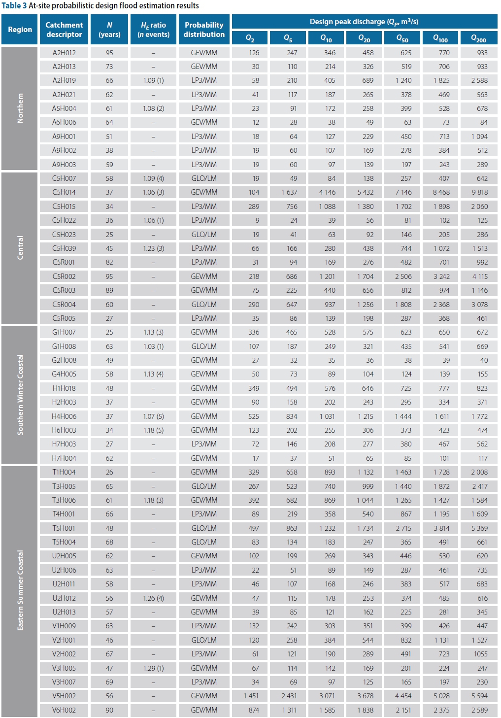
The at-site probabilistic design flood estimation results (Q_p) are presented in Table 3.

The average AMS record length of all the catchments listed in Table 3 is 56 years, while only 40 events (1.5%) of the 2 665 AMS events were being subjected to the H_Eextrapolations, as discussed in the Methodology section above. The statistical properties of each AMS dataset also confirmed the asymmetrical nature thereof, i.e. a high degree of variability and skewness. Consequently, the GEV/MM and LP3/MM probability distributions were regarded as the most suitable distributions in 46% and 38% of all the catchments, respectively. The GLO/LM probability distribution proved to be the most appropriate distribution in only 16% of all the catchments. The probabilistic plots based on the ranked AMS and Cunnane plotting position (Equation 1) at a catchment level in the four climatological regions are shown in Figures 2 to 5(b).

It is evident from Figures 2 to 5(b) that the dispersion about the mean (standard deviation) is relatively high in most of the catchments, while, due to the asymmetrical nature of each AMS, the lower tails of the probability distribution curves proved to be generally longer than the upper tails. At a regional level, the probabilistic curve fitting was dominated by LP3/MM distribution in the NR (Figure 2) and CR (Figure 3), while the GEV/MM distribution was the most appropriate in both the SWCR (Figure 4) and ESCR (Figures 5(a) and (b)). The use of the GLO/LM distribution was limited to the CR (three catchments), ESCR (four catchments), and SWCR (one catchment).

Overall, the above selection and use of theoretical probability distributions also proved to be in agreement with the general recommendations for at-site probabilistic flood frequency analyses in South Africa. For example, Alexander (2001) recommends only the LP3 distribution, Görgens (2007) recommends both the LP3 and GEV distributions, while Van der Spuy and Rademeyer (2016) extend their recommendation by including the LN distribution as well. The GLO/LM probability distribution is used extensively internationally as a standard procedure for flood frequency analysis, while LM parameter estimators could be used for the screening of discordant data and testing clusters for homogeneity (Smithers & Schulze 2000a). However, Alexander (2001) cautioned that LM parameter estimators are too robust against outliers, and emphasised that both low and high outliers are important characteristics of the flood peak maxima. The suppression of the effect of outliers could result in unrealistic estimates of higher return period values.

Estimation of catchment response time

A scatter plot of the catchment response times estimated using Equation 2 (USBR) and Equation 3 (G&S) is shown in Figure 6.

As shown in Figure 6, the r²value of 0.68 confirms the moderate degree of association between the catchment response times estimated using Equations 2 and 3, respectively. The USBR method's (Equation 2) slope (0.76), less than unity and negative y-inter-cept (-1.31), highlight that this method has an overall tendency to underestimate the T_cvalues in comparison to the G&S method (Equation 3). On average, Equation 2 underestimated the time of concentration with 46% in 38 catchments when compared to Equation 3, while an average overestima-tion of 36% is evident in the 10 remaining catchments. Such average differences in the catchment response time must be clearly understood in the context of the actual response time associated with the size of a particular catchment, as the impact thereof might be critical in a small catchment, while being less significant in a larger catchment. However, irrespective of the catchment size and/or differences in response time, these estimated T_cvalues will have a direct impact on both the estimates of design rainfall and peak discharge, all of which are elaborated on in the subsequent sections.

Estimation of design rainfall

A scatter plot of the design rainfall depths (p_T1and p_T2) associated with the T_c1and T_c2values in each catchment are shown in Figure 7.

It is evident from Figure 7 that the degree of association between the two DDF approaches decreases with an increasing return period, with the r² values ranging between 0.34 (T = 2-year) and 0.25 (T = 200-year). The modified Hershfield/ TR102 design rainfall depths were generally lower than the RLMA&SI design rainfall depths for T < 20-year. The frequency of these underestimations decreased with an increase in return period (e.g. 85% of the events at T = 2-year versus 50% of the events at T = 20-year), while the magnitude thereof remained relatively constant and varied between -21% and -25%. For T > 20-year, the opposite trend is evident. The modified Hershfield/TR102 design rainfall depths were generally higher than the RLMA&SI design rainfall depths, while the frequency of these overestimations increased with an increase in return period (e.g. 50% of the events at T = 20-year versus 61% of the events at T = 200-year). The latter overestimations remained relatively constant and varied between 11% and 19%.

The above differences, evident between the two DDF approaches, are most likely attributed to: (i) the longer record lengths and stringent data quality control procedures used in the RLMA&SI approach, and (ii) the different approaches to design rainfall estimation used, i.e. a single site approach (Adamson 1981) versus a regional approach (Smithers & Schulze 2003; 2004).

Furthermore, inconsistencies between the estimated 24-hour event values estimated using Equation 4 (modified Hershfield equation) and the TR102 1-day design rainfall information, on which the equation is based, were also evident. According to Smithers and Schulze (2003), the latter inconsistencies are ascribed to the fact that the functional relationship of Equation 4 does not accommodate the curvilinear relationship between design rainfall depth and log-transformed duration as applicable to most rainfall stations.

The above differences in design rainfall depths using the two different DDF approaches are truly appreciated when converted into design rainfall intensities, i.e. underestimated time parameters would result in higher design rainfall intensities, while the overestimation of time parameters is associated with lower design rainfall intensities. Both these scenarios would have a direct impact on the estimation of design floods, as detailed in the next section.

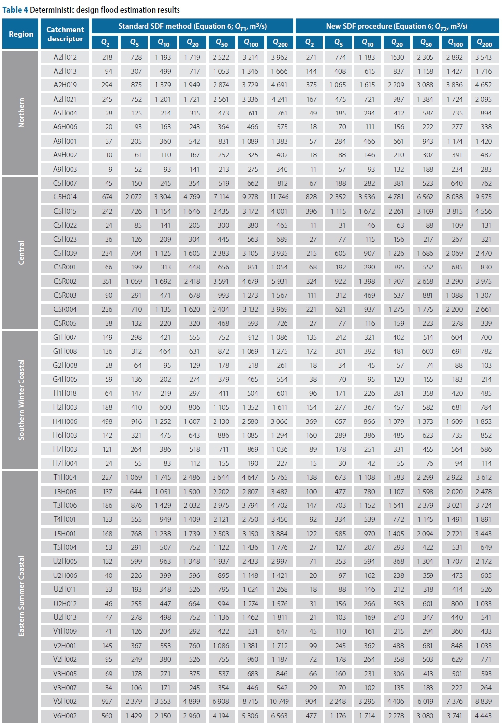
Estimation of deterministic design floods

The SDF design flood estimation results (Equation 6; Q_t1and Q_t2) are presented in Table 4, while the peak discharge ratios estimated using Equation 7 are shown in Figures 8(a) to 8(e).

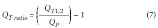
Where:

Q_T-ratio= peak discharge ratio (positive = overestimation and negative = underestimation) Q_t1= design peak discharge (m³/s) estimated using the standard SDF method

Q_t2= design peak discharge (m³/s) estimated using the new SDF procedure

Q_p= at-site probabilistic design peak discharge (m³/s)

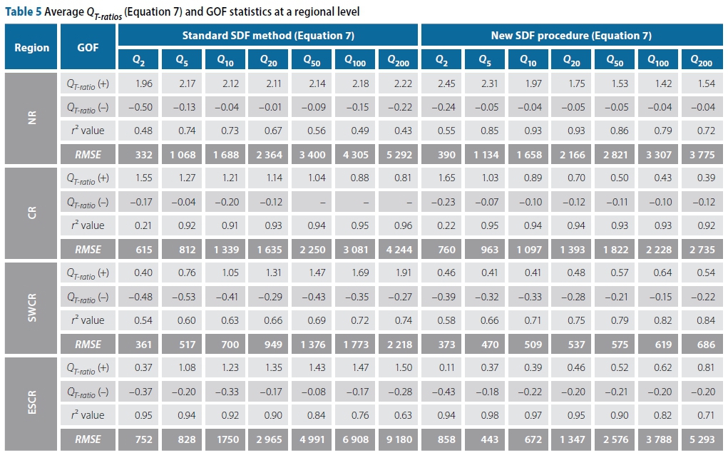
A summary of the goodness-of-fit (GOF) statistics based on the comparison between the at-site probabilistic design floods (Qp; Table 3) and the SDF design floods (Table 4) is listed in Table 5. The root mean square error (RMSE) is specifically included in Table 5 to ensure that the accumulated over- and/or underestimations are accounted for, i.e. to highlight the actual size (not source or type) of errors produced by the two SDF procedures, with the objective function to minimise the RMSE to zero.

The results contained in Tables 4 and 5, as well as Figures 8(a) to 8(e), are indicative of several trends associated with specific catchments and return periods, which are highlighted below:

■ Northern Region (SDF basins 1-3, Figure 8(a)): The SDF flood peaks (Q_T1 and Q_t2) exceeded the at-site probabilistic flood peaks (Qp) in all the catchments, except for catchments A9H002 and A9H003 in SDF basin 3. In 56% of all the catchments considered, the new SDF procedure (Q_T2,Equation 6) resulted in improved estimates in comparison to the standard SDF method (Q_T1, Equation 6) when compared to the at-site probabilistic flood estimates, especially in catchments A2H021 and A6H006. In the latter catchments, the standard SDF method (Q_T1, Equation 6) overestimated the at-site probabilistic flood peaks with between 62% and 653%, whereas the new SDF procedure's overestimations are limited to 300%. On average, the new SDF procedure (Q_T2, Equation 6) demonstrated the best results, especially for the higher return periods (e.g. T = 10-200-year; 142%-175% overestimation, < 5% underestimation, 0.72 < r² < 0.93, and 1 658 < RMSE < 3 775).

■ Central Region (SDF basin 9, Figure 8(b)) The standard SDF flood peaks (Q_T1) exceeded the at-site probabilistic flood peaks (Q_p) in all the catchments, except for the lower return periods (T < 20-year) in catchments C5H014 and C5R004. In more than 80% of all the catchments considered, the new SDF procedure (Q_T2, Equation 6) resulted in improved estimates in comparison to the standard SDF method (Q_T1, Equation 6) when compared to the at-site probabilistic flood estimates. The standard SDF method (Q_T1, Equation 6) overestimated the at-site probabilistic flood peaks with between 3% and 323%, whereas the new SDF procedure's overestimations are limited to 264%. However, in catchment C5H014, both the standard SDF method and new SDF procedure overestimated the at-site probabilistic flood peaks by a factor > 5 for T = 2-year. For all other return periods, the new SDF procedure (Q_T2, Equation 6) demonstrated the best average results (39%-165% overestimation, < 12% underestimation, 0.92 < r²< 0.95, and 963 < RMSE < 2 735).

■ Southern Winter Coastal Region (SDF basins 17 and 18, Figure 8(c)): The new SDF procedure (Q_T2, Equation 6) resulted in improved estimates in comparison to the standard SDF method (Q_T1, Equation 6) when compared to the at-site probabilistic flood estimates in all the catchments, except in catchment G1H007 where both methods had a tendency to underestimate the at-site probabilistic flood peaks with between 20% and 60%. In all other catchments and corresponding return periods, the new SDF procedure (Q_T2, Equation 6) demonstrated the best average results (41%-64% overestimation, 15%-39% underestimation, 0.58 < r²< 0.84, and 373 < RMSE < 686).

■ Eastern Summer Coastal Region (SDF basins 23-26, Figures 8(d)-8(e)): The new SDF procedure (Q_T2, Equation 6) resulted in improved estimates in comparison to the standard SDF method (Q_T1, Equation 6) when compared to the at-site probabilistic flood estimates in all the catchments, except for the two-year return period. The new SDF procedure (Q_T2, Equation 6) demonstrated better average results (11%-81% overestimation, 18%-43% underestimation, 0.71 < r²< 0.98, and 443 < RMSE < 5 293) than the standard SDF method, i.e. 37%-150% overestimation, 8%-37% underestimation, 0.63 < r²< 0.95, and 752 < RMSE < 9 180. Overall, the new SDF procedure (Q_T2, Equation 6) resulted in improved estimates in comparison to the standard SDF method (Q_T1, Equation 6) when compared to the at-site probabilistic flood estimates in more than 80% of all the catchments in the four climatological regions. Such improvements in design flood estimation also confirm that catchment response time and design rainfall are fundamental inputs to design flood estimation in ungauged catchments. However, despite the improvement in design flood estimation achieved in this study, the high over- and/or underestimations are still regarded as unacceptable and indicative that neither design rainfall nor catchment response time in these catchments could be regarded as the only fundamental input to design flood estimation. In essence, catchment response time should be regarded as enigmatic, since, although it is assumed to be an independent time parameter, it is actually dependent on the peak discharge, which in turn is also dependent on the design rainfall. Therefore, the latter over-and/or underestimations could also be ascribed to the regional SDF runoff coefficients not being representative of the average catchment conditions and/or physical regional descriptors.

The term 'runoff coefficient' is commonly used in flood hydrology (Young et al 2009; SANRAL 2013; Van der Spuy & Rademeyer 2016) to represent the percentage of effective rainfall that is transformed to direct runoff. Runoff coefficients vary substantially with the time scale of aggregation, i.e. in small catchments (< 15 km²) runoff coefficients represent an overall cutoff threshold separating effective rainfall from total rainfall and are readily obtainable from lookup tables, whereas in larger rural catchments, the runoff coefficients are normally associated with land use, soils and catchment slopes (Efstratiadis et al 2014). In both cases, these runoff coefficients are regarded as constant; however, it is obvious that its value depends both on the antecedent soil moisture conditions and on the rainfall intensity. To overcome this shortcoming, larger runoff coefficients are normally assigned to higher return periods, i.e. runoff coefficients increase as the return period increases, but such recommendations are not based on systematic investigations and favour arbitrary choices (Efstratiadis et al 2014).

Despite the simplicity of estimating runoff coefficients, it is evident that runoff coefficients play a secondary role in the overall predictive capacity of most deterministic design flood estimation methods in ungauged catchments. Hence, several modifications, e.g. modified runoff coefficients (Pegram 2003) and probabilistic approaches (Alexander 2002; Calitz & Smithers 2016), were suggested locally and abroad (Pilgrim & Cordery 1993) to deviate from a deterministic to a more probabilistic-deterministic approach. The SDF method is a typical example thereof, but due to several design limitations - i.e. regionalisation scheme adopted, lack of testing for homogeneity, outdated design rainfall information (TR102), etc - the method generally proved to be too conservative (Gericke & Du Plessis 2012). However, by using the more appropriate design rainfall information and catchment response times as input to the SDF method (this study), the results improved accordingly. In doing so, the variation of runoff coefficients with return period is also incorporated. Thus, as the intensity and volume of rainfall increases, the effect of the internal storage of catchments decreases, which leads to an increase in the runoff coefficients.

Typically, the large proportional differences between the c₂and c₁₀₀runoff coefficients (Equation 6), highlight that the SDF method assumes that a larger proportion of rainfall would contribute to the flood peaks and acknowledge that the antecedent soil moisture status of a catchment introduces additional variability into the rainfall-runoff process. However, variability increases with an increase in catchment size; hence, the difficulty to successfully establish a relationship between regional/ catchment descriptors and runoff coefficients in larger catchments. Hydrological literature, e.g. Pilgrim and Cordery (1993), Parak and Pegram (2006), and Gericke and Du Plessis (2012) also confirmed the latter and concluded that runoff coefficients are essentially functions of the return period and catchment response time.

 

CONCLUSIONS

The overall objective of this study was to independently test and compare the latest catchment response time and design rainfall estimation methodologies with current well-known and simplified methodologies used in South Africa to ultimately highlight the impact thereof on design flood estimation.

Building upon the critical assessment of available definitions, estimation procedures and the results from this study, it is evident that catchment response time, design rainfall, and to some lesser extent runoff coefficients, are key input parameters for design flood estimation in ungauged catchments, and have a significant impact on the design of hydraulic structures. Typically, high runoff coefficients, underestimated time parameters and associated lower design rainfall depths, although of much higher intensities, would result in over-designed hydraulic structures, while low runoff coefficients and overestimated time parameters would result in underdesigns. Not only will hydraulic structures be over-or underdesigned, but associated socioeconomic implications might render some projects as not being feasible, while any loss of life due to excessive flood damages and insufficient infrastructure is not excluded.

It is recommended that the current well-known and simplified catchment response time (USBR T_cequation) and design rainfall (modified Hershfield/TR102 DDF approach) estimation methodologies should be replaced with the empirical G&S T_cequations and the RLMA&SI DDF approach when deterministic design floods are estimated in ungauged catchments in South Africa. However, since the G&S T_cequations (Equation 3) are limited to only four climatological regions in South Africa, the further refinement thereof in terms of calibration, verification and possible regionalisation in other regions, is acknowledged. The proposed new SDF procedures are recommended for the estimation of flood peaks with return periods in excess of and including 10 years (T >10 years). In order to improve the depth of hydrological runoff data in South Africa, it is recommended that flow records be obtained from the DWS and verified. The verified data can then be utilised to improve on the findings in this study and to refine methods to be used for the purpose of design flood estimations, including those for T < 10 years.

Furthermore, the current research initiative of Calitz and Smithers (2016), which focuses on the development and assessment of regional runoff coefficients to be incorporated in the Probabilistic Rational Method (PRM) for South Africa, should be supported and welcomed by all research academic institutions and engineering practitioners involved in modern flood hydrology practice.

 

ACKNOWLEDGEMENTS

Support for this research by the National Research Foundation (NRF), University of KwaZulu-Natal (UKZN) and Central University of Technology, Free State (CUT) is gratefully acknowledged. I also wish to thank the anonymous reviewers of this paper for their constructive review comments, which have helped to significantly improve the paper.

 

REFERENCES

Adamson, P T 1981. Southern African storm rainfall. Technical Report TR102. Pretoria: Department of Environmental Affairs and Tourism.         [ Links ]

Alexander, W J R 2001. Flood risk reduction measures: incorporating flood hydrology for Southern Africa. Pretoria: University of Pretoria, Department of Civil and Biosystems Engineering.         [ Links ]

Alexander, W J R 2002. The standard design flood. Journal of the South African Institution of civil Engineering, 44(1): 26-30.         [ Links ]

Bondelid, T R, McCuen, R H & Jackson, T J 1982. Sensitivity of SCS models to curve number variation. Water Resources Bulletin, 20(2): 337-349.         [ Links ]

Calitz J P & Smithers J C 2016. Development and assesment of a probabilistic Rational Method for design flood estimation in South Africa. WRC Inception Report No K5/2748. Pretoria: Water Research Commission.         [ Links ]

DWAF (Department of Water Affairs and Forestry) 1995. GIS data: drainage regions of South Africa. Pretoria: DWAF.         [ Links ]

Efstratiadis, A, Koussis, A D & Mamassis, N 2014. Flood design recipes vs. reality: can predictions for ungauged basins be trusted? Natural Hazards and Earth System Sciences, (14): 1417-1428. DOI: 10.5194/nhess-14-1417-2014.         [ Links ]

Gericke, O J & Du Plessis, J A 2011. Evaluation of critical storm duration rainfall estimates used in flood hydrology in South Africa. Water SA, 37(4): 453-470. DOI: 10.4314/wsa.v37i4.4.         [ Links ]

Gericke, O J & Du Plessis, J A 2012. Evaluation of the standard design flood method in selected basins in South Africa. Journal of the South African Institution of civil Engineering, 54(2): 2-14.         [ Links ]

Gericke, O J & Du Plessis, J A 2013. Development of a customised design flood estimation tool to estimate floods in gauged and ungauged catchments. Water SA, 39(1): 67-94. DOI: 10.4314/wsa.v39i1.9.         [ Links ]

Gericke, O J & Smithers, J C 2014. Review of methods used to estimate catchment response time for the purpose of peak discharge estimation. Hydrological Sciences Journal, 59(11): 1935-1971. DOI: 10.1080/02626667.2013.866712.         [ Links ]

Gericke, O J & Smithers, J C 2016a. Are estimates of catchment response time inconsistent as used in current flood hydrology practice in South Africa? Journal of the South African Institution of civil Engineering, 58(1): 2-15. DOI: 10.17159/2309-8775/2016/v58n1a1.         [ Links ]

Gericke, O J & Smithers, J C 2016b. Derivation and verification of empirical catchment response time equations for medium to large catchments in South Africa. Hydrological processes, 30(23): 4384-4404. DOI: 10.1002/hyp.10922.         [ Links ]

Gericke, O J & Smithers, J C 2017. Direct estimation of catchment response time parameters in medium to large catchments using observed streamflow data. Hydrological processes, 31(5): 1125-1143. DOI: 10.1002/hyp.11102.         [ Links ]

Grimaldi, S, Petroselli, A, Tuaro, F & Porfiri, M 2012. Time of concentration: a paradox in modern hydrology. Hydrological Sciences Journal, 57(2): 217228. DOI: 10.1080/02626667.2011.644244.         [ Links ]

Görgens, A H M 2007. Joint Peak-Volume (JPV) design flood hydrographs for South Africa. WRC Report No 1420/3/07. Pretoria: Water Research Commission.         [ Links ]

Kerby, W S 1959. Time of concentration for overland flow. civil Engineering, 29(3): 174.         [ Links ]

McCuen, R H 2005. Hydrologic Analysis and Design, 3rd ed. Upper Saddle River, NJ: Prentice-Hall.         [ Links ]

McCuen, R H, Wong, S L & Rawls, W J 1984. Estimating urban time of concentration. Journal of Hydraulic Engineering, 110(7): 887-904.         [ Links ]

Midgley, D C & Pitman, W V 1978. A Depth-Duration-Frequency diagram for point rainfall in Southern Africa. HRU Report No 2/78. Johannesburg: University of the Witwatersrand, Hydrological Research Unit.         [ Links ]

Midgley, D C, Pitman, W V & Middleton, B J 1994. Surface water resources of South Africa. WRC Report No 298/2/94. Pretoria: Water Research Commission        [ Links ]

Parak, M & Pegram G G S 2006. Rational formula from Runhydrograph. Water SA, 32(2): 163-180.         [ Links ]

Pegram, G G S 2003. Rainfall, Rational Formula and Regional Maximum Flood - Some scaling links. Australian Journal of Water Resources, 7(1): 29-39.         [ Links ]

Pegram, G G S & Parak, M 2004. A review of the Regional Maximum Flood and Rational Formula using geomorphological information and observed floods. Water SA, 30(3): 377-392.         [ Links ]

Pilgrim, D H & Cordery, I 1993. Flood runoff. In: Maidment, D R (Ed.). Handbook of Hydrology. New York: McGraw-Hill, Ch 9, 1-42.         [ Links ]

Pullen, R A 1969. Synthetic unitgraphs for South Africa. HRU Report No 3/69. Johannesburg: University of the Witwatersrand, Hydrological Research Unit.         [ Links ]

Rahman, A, Weinmann, P E, Hoang, T M T & Laurenson, E M 2002. Monte Carlo simulation of flood frequency curves from rainfall. Journal of Hydrology, 256: 196-210.         [ Links ]

SANRAL (South African National Roads Agency Limited) 2013. Drainage Manual, 6th ed. Pretoria: SANRAL.         [ Links ]

Schmidt, E J & Schulze, R E 1984. Improved estimation of peak flow rates using modified SCS lag equations. ACRU Report No 17. Pietermaritzburg: University of Natal, Department of Agricultural Engineering.         [ Links ]

Seybert, T A 2006. Stormwater management for land development: methods and calculations for quantity control. Hoboken, NJ: Wiley.         [ Links ]

Smithers, J C 2012. Review: Methods for design flood estimation in South Africa. Water SA, 38(4): 633-646.         [ Links ]

Smithers, J C & Schulze, R E 2000a. Development and evsaluation of techniques for estimating short duration design rainfall in South Africa. WRC Report No 681/1/00. Pretoria: Water Research Commission.         [ Links ]

Smithers, J C & Schulze, R E 2000b. Zong duration design rainfall estimates for South Africa. WRC Report No 811/1/00. Pretoria: Water Research Commission.         [ Links ]

Smithers, J C & Schulze, R E 2003. WRC Report No 1060/01/03. Design rainfall and flood estimation in South Africa. Pretoria: Water Research Commission.         [ Links ]

Smithers, J C & Schulze, R E 2004. The estimation of design rainfall for South Africa using a regional scale invariant approach. Water SA, 30(4): 435-444.         [ Links ]

USBR (United States Bureau of Reclamation) 1973. Design of Small Dams, 2nd ed. Washington, DC: Water Resources Technical Publications.         [ Links ]

USDA NRCS (United States Department of Agriculture, Natural Resources Conservation Service) 2010. Time of concentration. In: Woodward, D E (Ed.) National Engineering Handbook. Washington, DC: USDA NRCS, Ch 15, Section 4, Part 630, 1-18.         [ Links ]

Van der Spuy, D & Rademeyer, P F 2016. Flood frequency estimation methods as applied in the Department of Water and Sanitation. Pretoria: Department of Water and Sanitation.         [ Links ]

Van Vuuren, S J, Van Dijk, M & Coetzee, G L 2012. Status review and requirements of overhauling flood determination methods in South Africa. WRC Report No K8/994/1. Pretoria: Water Research Commission.         [ Links ]

Wilson, E M 1990. Engineering hydrology, 4th ed. London: Macmillan.         [ Links ]

Young, C B, McEnroe, B M & Rome, A C 2009. Empirical determination of rational method runoff coefficients. Journal of Hydrologic Engineering, (14): 1283-1289.         [ Links ]

 

 

Correspondence:
O J Gericke
Unit for Sustainable Water and Environment
Department of Civil Engineering
Central University of Technology, Free State
Private Bag X20539, Bloemfontein 9300, South Africa
T: +27 51 507 3516 / +27 73 582 6812
E: jgericke@cut.ac.za

 

 

 

DR JACO GERICKE Pr Eng graduated with B Tech Eng (Civil) and M Tech Eng (Civil) degrees from the Central University of Technology, Free State (CUT). He was also awarded the BSc (Hons) Appl Sci Water Resources Eng degree by the University of Pretoria, the MSc Eng (Civil) degree by Stellenbosch University and a PhD Eng (Agriculture) degree by the University of KwaZulu-Natal. He has 20 years of professional and academic experience, and has published a number of papers in the design hydrology field. He is currently a Senior Lecturer at the CUT.