


Serviços Personalizados
Artigo
 Inglês (pdf)
 Artigo em XML
 Referências do artigo
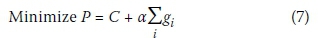
Indicadores

Links relacionados
-
 Citado por Google
 -
 Similares em Google
Compartilhar

 Permalink
Journal of the South African Institution of Civil Engineering
versão On-line ISSN 2309-8775
versão impressa ISSN 1021-2019
J. S. Afr. Inst. Civ. Eng. vol.60 no.3 Midrand Set. 2018
http://dx.doi.org/10.17159/2309-8775/2018/v60n3a1
TECHNICAL PAPER
Sewer network design layout optimisation using ant colony algorithms
N de Villiers; G C van Rooyen; M Middendorf
ABSTRACT
The optimal design of sewer networks typically comprises two sub-problems. The first is to determine an optimal layout of the network elements, and the second to optimally design the network components. In this article the focus is on the optimisation of gravity sewer network layouts, which requires simultaneous optimisation of hydraulic design. The layout is optimised using ant colony algorithms with four proposed node and edge-based selection strategies, while a heuristic optimisation algorithm is used for the hydraulic optimisation. The resulting simultaneous optimisation algorithm is shown to perform very well. The selection strategies are shown to be effective, but no clear best strategy is identified, as the performance of the layout algorithms is shown to depend heavily on characteristics of the network under consideration. However, some strategies are shown to perform inconsistently and worse than others on average.
Keywords: gravity sewer network, ant colony optimisation, tree-growing algorithm, layout optimisation, graph theory
INTRODUCTION
The optimisation of sewer networks typically consists of two sub-problems. The first is to determine the layout of network elements and the second to determine all hydraulic parameters - such as diameters, slopes, etc - of the network components. The two sub-problems of the optimisation are strongly linked - for each layout a unique set of hydraulic parameters exists. Consequently, if an optimal design is to be found, the sub-problems have to be solved simultaneously. However, this does not mean that a single selection strategy or algorithm has to be used for both subproblems. Rather, the fitness of a solution should be determined based on both layout and component sizes simultaneously. Due to the complexity of such algorithms, most research has been done on one of the subproblems, while the other remains static, usually the layout (Lejano 2006).
There are three approaches to simultaneous layout and element sizing optimisation:
1. Complete enumeration
In this approach all feasible layouts are generated and the hydraulic design of each is completed individually (Diogo et al 2000; Diogo & Graveto 2006). While this approach is very useful for finding the best layout, its application is only practical for small-scale problems.
2. Separated design
This approach separates the two design problems, either through manual layout design or by using individual objective functions for each sub-problem. Once the optimal layout is found, the optimal hydraulic parameters for this layout is determined by a separate algorithm (Pan & Kao 2009; Haghighi 2013). While this approach is useful for large problems, it is difficult to determine true optima (Haghighi & Bakhshipour 2015).
3. Simultaneous design
The layout and element size problems are optimised simultaneously (Li & Matthew 1990; Moeini & Afshar 2012; Haghighi & Bakhshipour 2015). While this approach is the most promising in finding true global optima for large solutions its implementation is the most complex and requires complex formulation and specific design algorithms (Haghighi & Bakhshipour 2015). The fitness of a solution is calculated taking both layout and hydraulic parameters into account simultaneously.
In this work the third approach (simultaneous design) is used to develop a hybrid Ant Colony Optimisation (ACO) algorithm by which the layout and all hydraulic parameters are simultaneously optimised. For each individual layout created by the ACO algorithm the set of hydraulic parameters is optimised. The two sub-problems of sewer network optimisation are very different mathematically. The hydraulic design problem is a non-linear discrete programming problem, while the layout problem is a variant of the degree-constrained Minimum Spanning Tree (d-MST) problem in graph theory. In this article development of the layout optimisation algorithm and combining of the algorithm with the heuristic hydraulic optimisation procedure proposed by De Villiers et al (2017) to create a hybrid algorithm capable of solving both subproblems simultaneously, are addressed.
MODELLING SEWER NETWORKS USING GRAPH THEORY
In this investigation graph theory is used to model the layout of sewer networks. Layout design of sewer networks is again a two-part problem. The first is to determine the spatial location of manholes and pipes. The second is to determine the direction of flow of each pipe. A full network layout is only found once both parts of the problem have been solved.
Spatial design of the network
Referring to Figure 1, the nodes, representing manholes labelled 1, 2, 3 and 4 respectively, are connected by edges, representing pipes labelled 1, 2, 3, 4 and 5 respectively.
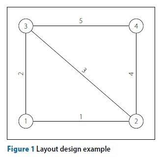
In this example the spatial positions of the manholes and pipes have already been determined, i.e. the first part of the design is complete. However, it may have been equally feasible to place the manholes at different locations and to connect them differently, for example by placing pipe 3 between manholes 1 and 4 rather than 2 and 3. This part of the design, deciding on the spatial location of manholes and how to connect them with pipes, is most often governed by existing or planned infrastructure, such as roads or buildings, and topographical considerations, such as hills or steep inclines. In this paper it is assumed that the positioning of manholes and pipes is completed prior to the optimisation process aimed at minimising the installation cost of the sewer network. The positioning of manholes and pipes is referred to as the base layout, or base graph of the layout. All pipes and manholes included in the base graph must be present in the final solution. The base layout is modelled mathematically as an undirected graph where the vertices represent manholes and the edges pipes:
Gbase = (V E)
Where:
Gbase= the base graph
V = the vertex set, whose elements are the vertices of Gbase which represent manholes of the sewer network
E = the edge set, whose elements are the edges of Gbase which represent pipes of the sewer network. As the graph Gbase is undirected, the individual edges are unordered pairs (u, v) where u and v are vertices in V.
Directional design of the network
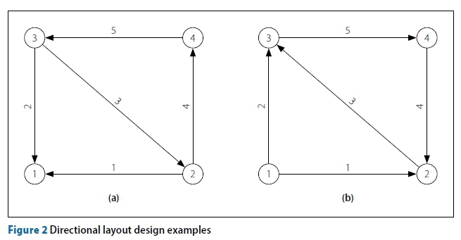
The second part of the layout design is to determine the direction of flow for each pipe. This part of the layout design is deceptively complex, and the number of possible permutations grows exponentially as the number of vertices and edges in the base graph increases. This part of the layout design is the concern of the optimisation procedures which are discussed in detail in the section below titled "Objective function" on page 9. A brief overview of the required decisions to complete the directional design is given here. Figure 2 shows two directional graphs (directions are indicated by arrows).
Figure 2 shows two feasible final layouts of a possible 52 = 25 of the base layout shown in Figure 1. The choice of flow directions can heavily influence the final capital investment cost of the completed sewer network, especially when adverse topographical conditions are present. If, for example, manhole 2 has a much lower elevation than manhole 3, then using sound engineering intuition we can readily observe that the design of Figure 2(a) requires less excavation than that of Figure 2(b). This reduction in required excavation can be expected to lead to a reduction in capital expenditure. However, the problem becomes increasingly difficult as the size of the base graph increases, since the change in flow direction of a single pipe may have significant effects on the cumulative downstream flow rates within pipes, and therefore their required diameters and slopes.
Notice that in both designs in Figure 2, cycles are present in the final layout designs. For Figure 2(a) the cycle 2-4-3 exists and for Figure 2(b) the cycle 2-3-4 exists. In this investigation only gravity sewer networks are considered, with no special structures present, such as divergence structures, pumping stations or rising mains. This implies that all manholes may only have a single outgoing pipe, often referred to as the single out-degree constraint. These assumptions drastically simplify the hydraulic analysis of the network.
Moeini and Afshar (2012) propose disconnecting pipes from their upstream manholes and creating what they term adjacency nodes, which are created artificially at the same location as the existing upstream manhole. The practical implication of this is that the pipe has no upstream inflow from the manhole, and cycles are removed from the network. Referring to Figure 3, the networks shown are similar to those in Figure 2. In this case, however, some pipes have been disconnected from their upstream manholes and adjacency nodes created, indicated by perpendicular lines on the upstream end of the pipe.
Constraints on the optimisation problem
De Villiers et al (2017) provide an overview of sewer network design, and all constraints and equations described there are applicable to this paper. When constructing a network layout, however, the single out-degree constraint, described above, has to be considered. This avoids cycles and diversion structures, and the resulting layout is a simple branched gravity sewer network with no special structures.
To ensure that any proposed layout adheres to these simplifications, only branched network layouts are selected from the power set of the base layout, which contains all possible looped and branched layouts. Mathematically the restrictions for a branched layout in a network with M manholes are (Moeini & Afshar 2012):
Where:
This constraint is augmented with the continuity requirement at each node j:
Where:
= flow rate in pipe i between nodes l and j with either node as source or target
s = the outlet node
The network is defined with a single outlet in this paper. The continuity equation is not enforced at the outlet, since only the inflow is modelled for the outlet node. Note that this restriction does not affect the generality of the proposed method, since the same method may be applied for multiple outlets simultaneously.
ANT COLONY OPTIMISATION
ACO algorithms have been successfully applied to various constrained optimisation problems, and achieve state-of-the-art results for several important problem classes, such as the Quadratic Assignment Problem (QAP) and scheduling and routing (Dorigo & Stützle 2004) to name a few. The precursor algorithm to all ACO algorithms, Ant System (AS), was inspired by observing the phero-mone-based trail-laying-trail-following of real ants (Dorigo et al 1996). Though modern ACO algorithms have come a long way from the initial AS model, the analogy of a colony of foraging ants is still useful in understanding the behaviour of the algorithm.
In ACO a number of individual ants each generates solutions independently and in parallel, over many iterations. The ants make decisions using a so-called 'phero-mone-value', which models the fitness of an eligible decision at a decision point. The best solution in an iteration is used for trail-laying, i.e. the pheromone value is increased along the best trail, while some pheromone on all other trails is evaporated. Through this process of pheromone deposition and evaporation the search near good solutions is intensified over time,
while initially maintaining diversity within the search space. The steps of a general ACO algorithm are now described (Dorigo et al 1996):
1. Select a suitable size for the set of ants {A}kfor each generation k and set initial pheromone values on all available selections to some suitable, but equal, value. Set generation count k = 0.
2. Starting from either a predetermined or randomly selected point, construct a solution for each individual ant, a Є {A}kof the current generation, using the standard transition rule to make a decision:
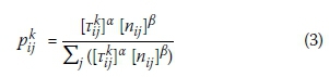
Where:
k = the generation number
= probability of decision j at decision point i, hereafter "decision ij" in generation k
= pheromone value of decision ij in generation k
= heuristic influence value at decision ij
α = relative pheromone influence factor
β = relative heuristic influence factor
3. Using a problem-specific objective function, determine the fitness f(a) of each ant's solution, a Є {A}k.
4. Acquire the generation-best solution f(best)*. Compare acquired generation best solution to current global best solution f(best)global, replacing the global best if the generation best solution is better.
5. Perform pheromone evaporation on all paths and increase the pheromone along the path selected by the generation-best solution, using the following update rule:
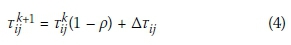
with p the evaporation rate and ATijthe pheromone increase of the generation-best solution, defined as:
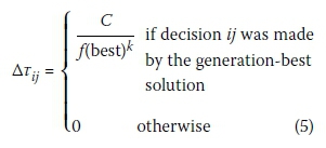
Where:
C = a constant real number
6. Check convergence of the algorithm. Usually convergence is accepted if a minimum number of generations have been completed, and for a number of generations thereafter the global-best solution has not improved. Alternatively, if all individuals of a generation produce the same solution, the algorithm has converged. If the algorithm has converged, accept current global-best solution as final solution, otherwise return to step 2 and repeat the process.
Many modifications have been proposed in the literature to improve the behaviour of the ACO algorithm. The modifications used in this implementation and their effects are now described.
-
Changing the evaporation rate. The evaporation rate p determines the convergence speed of the algorithm. In general, when a large search space is to be investigated a low value of p is beneficial, since the algorithm will be allowed more time to explore the different regions of the search space before focusing on a small region (Merkle et al 2002). Merkle et al (2002) found that, when the maximum number of iterations is restricted, a higher value of p usually performs better. Therefore it is proposed by Merkle et al (2002) that two different values of p be used during the run of an ACO algorithm. Initially, a low p is used which remains constant for the majority of the generations. For the last generations of the algorithm a high p value is used to perform a final intensive search near the best solution that has been found.
-
Modified elitist strategy. Using an elitist strategy is a common modification to ACO algorithms. This entails using a pheromone update from both the generation-best and current global-best solution at the end of each generation. The pheromone update rule is modified to reflect this:
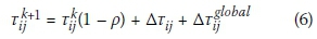
The elitist strategy has the advantage that the search is intensified around the current global-best solution. However, if the global-best solution remains unchanged for many generations it has a great influence on the pheromone values which may, during long runs, cause the algorithm to converge prematurely to the current global-best solution (Merkle et al 2002). This is especially true if the current global-best solution is a single good solution, with no other good solution in the neighbourhood. It is therefore proposed (Merkle et al 2002) to set a maximum number of generations, gmax, during which an elitist solution is allowed to remain unchanged. When the elitist solution has exceeded its maximum number of generations it is replaced by the current generation's best solution, even if this solution is worse than the current global-best. The replacement is only in terms of pheromone updates; the solution is, however, retained as the current best solution of the optimisation. When an elitist solution has good solutions in its neighbourhood it is likely the ants will discover it within reasonable time. Otherwise it does not matter that the elitist solution has been discarded, as no improved solutions are in its neighbourhood.
LAYOUT OPTIMISATION
Layout optimisation of a sewer network is one part of the two-part network optimisation problem, in which the flow direction of pipes has to be determined for a given base layout. This part of the problem has been studied less than the hydraulic optimisation problem. However, some researchers have proposed algorithms for the simultaneous solution of both subproblems. Walters (1985) used Dynamic Programming (DP) for simultaneous layout and size optimisation, and his method could be used to drain a set of sources with fixed positions. Li and Matthew (1990) used Discrete Differential Dynamic Programming (DDDP), which utilised an iterative procedure to generate the layout, and then to size the sewers and pumps while keeping the layout fixed. DDDP has some significant drawbacks - it restricts the search space and reduces the probability of locating the global optimum. The DDDP stages must be manually divided for each individual problem and this reduces its practicability. Pan and Kao (2009) used a Genetic Algorithm (GA) combined with Quadratic Programming (QP). In their approach a majority of the constraints were formulated in QP, while other parameters, such as layout and pipe diameters, were determined by the GA. Moeini and Afshar (2012) proposed an Ant Colony Optimisation (ACO) algorithm combined with a Tree Growing (TG) algorithm which performs both the layout construction and selects diameters simultaneously. In their approach it is assumed that all pipe flow rates are at maximum relative flow depth, allowing for the calculation of pipe slopes. Haghighi and Bakhshipour (2015) combined previous works, namely the loop-by-loop cutting algorithm (Haghighi 2013) and an Adaptive Genetic Algorithm (Haghighi & Bakhshipour 2012), with a Tabu Search (TS) algorithm to create an effective hybrid algorithm for simultaneous layout and element size optimisation.
Despite the suitability of ACO algorithms to the layout optimisation problem of sewer networks they have seen limited use. The main reason for this is the two-part nature of the problem. ACO algorithms require a significant number of function evaluations, for each of which both layout and hydraulic optimisation have to be performed simultaneously if the best results are to be obtained. Because of this the algorithm can be extremely computationally expensive. To overcome this problem Moeini and Afshar (2012) in their ACO-TG algorithm use the ants to simultaneously select both layout and diameter. This strategy, of using a single algorithm for both layout and diameter selections, is also employed by Pan and Kao (2009) in their GA-QP algorithm. The major disadvantage of this is the potential for fitness warping. If a very good layout is produced early on in the iterations, it is very likely that a poor set of diameters will be selected with it, and consequently the fitness of the entire network is compromised and the algorithm is unable to identify that a good layout has been found. In order to overcome fitness warping a separate optimisation algorithm is employed for each sub-problem in this paper. This approach, also used by Haghighi and Bakhshipour (2015) in their hybrid Tabu-Search algorithm, can be extremely computationally expensive. Haghighi and Bakshipour (2015) overcome the computational restrictions of this approach by using an efficient layout-generating algorithm combined with a relatively efficient meta-heuristic for element size optimisation. In this work, the computationally expensive ACO algorithm, combined with a TG algorithm as proposed by Moeini and Afshar (2012), is used to determine layouts and then combined with the computationally efficient heuristic optimisation algorithm developed by De Villiers et al (2017).
In this implementation the networks are restricted to gravity sewer networks. Additionally no cycles nor diversion structures are allowed within the network. This is achieved by restricting the out-degree, the number of outlet pipes, of each node to one. This assumption creates a variant of the d-MST problem, not simply because only the out-degree is constrained, but also because no clear definition of a minimum exists. The lack of a minimum definition means that traditional graph theory algorithms for minimum spanning tree construction, such as Prim's or Kruskal's algorithms, cannot be used without significant modifications. Bui and Zrncic (2006) showed that ACO algorithms perform well for the solution of d-MST problems. These applications offer valuable insights which may assist in understanding the nature of optimal layouts of sewer networks. Bau et al (2008) compared Prim's algorithm, which uses node-based selection, and Kruskal's algorithm, which uses edge-based selection, and found Kruskal's algorithm to be superior. Both node-based and edge-based layout creation strategies are developed and compared:
1. Edge-based selection which directly queries the base graph to construct a spanning tree, similar to Moeini and Afshar (2012) - henceforth referred to as the "direct-edge" strategy.
2. Node-based selection which directly queries the base graph to construct a spanning tree - henceforth referred to as the "direct-node" strategy.
3. Constructing a spanning tree using a permutation of unique edge identities - henceforth referred to as the "permutation-edge" strategy.
4. Constructing a spanning tree using a permutation of unique node identities - henceforth referred to as the "permutation-node" strategy.
For all the selection strategies above the hydraulic optimisation is performed by the Heuristic Optimisation Algorithm developed by De Villiers et al (2017). The hydraulic optimisation algorithm is deployed for each individual layout created by the layout creation algorithm to determine the optimal set of hydraulic parameters. Once the layout creation and hydraulic design are complete the fitness of the solution may be calculated using Equation 7.
Figure 1 shows a small example network's base layout, which will be used to describe the spanning tree construction strategies. The base layout, alternatively referred to as the base graph, of the network shows the position of all the manholes and all the pipes that are required in the network. Additionally, the elevations and design inflow rates at each manhole are known. The layout optimisation algorithm does not move the pipe around, but is rather used to determine the flow direction of pipes. In this example node 1 is the outlet node.
Figure 4 shows all the possible paths of nodes and edges for the example network in Figure 1. The nodes are shown in circles, while the edges which would result in the addition of the next node are shown in square brackets.
Figure 4 is not determined by using any of the selection strategies. This simply shows all the possible paths to follow to construct a spanning tree of this network. The selection strategies are employed to determine which decisions are eligible and decide how to present the eligible decisions at each point to the layout creation algorithm. For example, at the start the layout creation algorithm could be presented with either the eligible edges 1, 2, or the eligible nodes 2, 3. If edge 1, or node 2, was selected, then the eligible set of edges and nodes at the following iteration are 2, 3, 4 and 3, 4 respectively.
In an ACO that uses a single pheromone matrix, the ants can only make one choice based on the pheromone. If another choice has to be made, some mechanism, usually a heuristic, is required to resolve it. For the sewer network layouts, a useful parameter proposed my Moeini and Afshar (2012) is the hop-rank. This parameter ranks nodes based on the number of preceding nodes in its branch. Referring to Figure 1, if a spanning tree consisting of edges 1, 3 and 5 is assumed, the hop-ranks of nodes 1 through 4 are respectively 0, 1, 2 and 3. The hop-rank parameter can be used to favour selections which do not increase the length of already long branches. If required, the hop-rank parameter can be used to make a heuristic selection. In all cases no heuristic influence value nijis used, since that would render direct comparison of the effectiveness of the strategies impossible.
Direct-edge layout creation
This strategy mimics the edge selection behaviour of the algorithm proposed by Moeini and Afshar (2012). The tree-growing algorithm compiles a set of eligible edges, always starting from the static sink node. An edge is considered eligible for selection if only one of its vertices is already included in the growing spanning tree. The edge selection procedure is shown below.
1. Define:
T = the spanning tree
TN= the set of nodes in the spanning tree
E = the set of currently eligible edges
nt= the target node of the new edge
ns= the source node of the new edge
2. Initiate T and TN. Insert the sink node into TN.
3. Compile E, the set of all eligible edges; an edge is considered eligible if TN contains one of its nodes.
4. Select the next edge e of T from E using the transition rule described in the section titled "Ant Colony Optimisation" on page 4.
5. Identify ntand nsof e. Select nt, the target node, as the node already contained in TN and the other as ns.
6. Add e to T, add nsto TN.
7. If TN contains all nodes, stop. Or else return to 3.
Referring to Figure 4, if in the first iteration edge 1 was selected and in the second edge 2, then the set of eligible edges for iteration three would be E = {4; 5}. Edge 3 is not eligible since both its nodes are elements of TNand it would introduce a cycle into the network. The way in which edge 3 will be added to the network is described further down in the section titled "Layout completion" on page 8. Determining the source (upstream) and target (downstream) nodes of a selected edge is done simply by checking which node of the edge is already contained in TNand assigning that as the target.
Direct-node layout creation
In this strategy the tree-growing algorithm constructs sets of eligible source and target nodes. A node is considered to be an eligible source if any edge connected to it has a node which is already included in the growing spanning tree. This is best achieved by using the nodes already contained in the spanning tree as potential target nodes and finding their adjacency nodes, using the base graph that can serve as potential source nodes. The direct-node strategy is formally described below.
1. Define:
N = set of all nodes
T = the spanning tree
TN= set of nodes in the spanning tree
ei= eligible node i
E = set of currently eligible nodes
Ai= set of nodes adjacent to node i
ni= node being added to the spanning tree at current iteration
2. Initiate T and TN. Insert the sink node into TN.
3. Compile the set of eligible source nodes E. A node ei is considered eligible for selection if it is not already contained in TN and its set of adjacent nodes Aicontains at least one node already contained within TN.
4. Select the next node to be added to the growing spanning tree ni from E using the transition rule described in the section titled "Ant Colony Optimisation" on page 4. Add n¡to TN.
5. Find the eligible target nodes for the new edge, with nias its source node. Compile Ani, the set of nodes adjacent to node ni. Compile the set of eligible target nodes E. A node is considered eligible to be a target node if it is both an adjacent node of ni, i.e. an element of Ani, and currently contained in TN.
6. If E contains more than one element, select eifrom E with the lowest hoprank as the target node. If nodes have equal hop-ranks, make a random choice between them. Alternatively take the single element of E as the target node.
7. Add a new edge from the source node to the target node to T.
8. If TN contains all nodes, stop. Or else return to step 3.
The direct node strategy places some limitations on the networks that can be produced by the algorithm. Referring to Figure 1, if only edges 2 and 5 have been included in the growing spanning tree, only node 2 is eligible as the next source node. The set of eligible target nodes of node 2 is E = {1, 3, 4}. Due to the hop-rank heuristic it would only ever be possible to select node 1 as the target node.
Permutation-edge layout creation
The permutation strategies are used as alternatives to the previous methods in which the base graph is queried directly. In this case an ant colony algorithm is used to construct a permutation of unique edge identities from which a spanning tree of the base graph is eventually created. The steps that create the edge permutation are listed below.
1. Compile the set N of all base graph edges. Initialise permutation P = 0, the empty set.
2. Compile set of eligible edges E. An edge is considered eligible if it is not contained in P. If E = 0, stop.
3. Using the transition rule described in the section titled "Ant Colony Optimisation" on page 4, select the next edge ei from E to be added to the permutation. Concatenate eito the end of P.
4. Return to 2.
Once a permutation has been composed it can be used to construct a layout by simply using the order of the edges in the permutation as the order in which to add edges to a growing spanning tree. The permutation-edge layout construction, which is very similar to its direct-edge counterpart, is described below.
1. Define:
T = the spanning tree
P = the permutation
TN= the set of nodes in the spanning tree
E = set of currently eligible edges
nt= the target node of the new edge
ns= the source node of the new edge
2. Initiate T and TN. Insert the sink node into TN.
3. Compile E, the set of eligible edges. Similar to the direct-edge strategy, an edge is considered eligible if TN contains one of its nodes.
4. Iterate P. The first edge encountered in P which is also in E is selected as the next edge to add the T; however, it is not added to T at this point as its direction is only determined during the next step.
5. Identify the source node nsand target node ntof the new edge by selecting nt as the node which is already in TN. Now add the nsto TN.
6. Add e to T.
7. If TNcontains all nodes, stop. Or else return to 3.
Assume P = {12345}. Then, referring to Figure 1, after two iterations both edges 1 and 2 have been added and E = {4, 5}. Iterating through P encounters edge 4 prior to 5, so edge 4 is the next one to be added to the spanning tree.
Permutation-node layout creation
In this case spanning tree layouts are constructed using permutations of unique node identities. An ant colony algorithm is used to create the node permutations as described below.
1. Compile the set N of all base graph nodes. Initialise permutation P = 0, the empty set.
2. Compile set of eligible nodes E. A node is considered eligible if it is not contained in P. If E = 0, stop.
3. Using the transition rule described in the section titled "Ant Colony Optimisation" on page 4, select the next node eifrom E to be added to the permutation. Concatenate e to the end of P.
4. Return to 2.
From the node permutation a spanning tree can be constructed by adding nodes to the spanning tree in the same order that they appear in the permutation, as described below.
1. Define:
N = set of all nodes
T = the spanning tree
P = the permutation
TN= set of nodes in the spanning tree
ei= eligible node i
E = set of currently eligible nodes
Ai= set of nodes adjacent to node i
ni= node being added to the spanning tree in the current iteration
2. Initiate T and TN. Insert the sink node into TN.
3. Compile the set of eligible source nodes E. A node ei is considered eligible if it is not already contained in TN and its set of adjacent nodes Ai contains at least one node already contained in TN.
4. Iterate P. The first node ntencountered in P, which is also in E, is selected as the next source node to be added to the growing spanning tree. Add n¡ to TN.
5. Determine the target node for the new edge. Compile Ani-, the set of nodes adjacent to node ni. Compile the set of eligible target nodes E. A node is considered eligible as the target node if it is contained in both TN and Ani
6. If E contains more than one element, iterate over P. The first node nj encountered in the iteration, such that n is in E, is taken as the target for the new edge. Alternatively take the single element of E as the target node. Add njtoTN.
7. Add a new edge from the source node n¡_ to the target node n to T.
8. If TN contains all nodes, stop. Or else return to step 3.
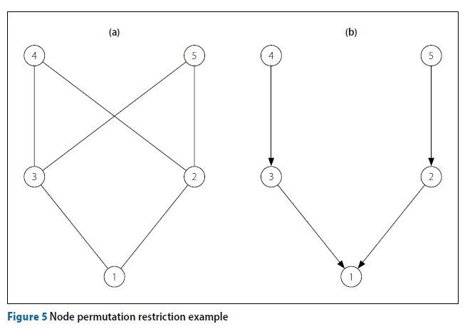
Note that in the direct-node method, the hop-rank heuristic was used to select the target node, while in this case the permutation is used to choose the target node by selecting the first node encountered in P which is also in E. This heuristic decision again places some restriction on the spanning trees that can be produced, as demonstrated using Figure 5. Figure 5(a) shows the base layout of a network, while Figure 5(b) shows a spanning tree of this network which cannot be created by the permutation-node approach. This is due to the fact that for node 4 to connect to node 3, rather than node 2, node 3 has to appear before node 2 in the permutation. Then, however, node 5 will also connect to node 3. The opposite is also true - if node 2 appeared before node 3 in the permutation, then both nodes 4 and 5 will connect to node 2.
Layout completion
Once a spanning tree has been created, all edges of the base graph that are not included in the spanning tree have to be added to complete the network. These edges have to be reintroduced in such a way that cycles are not formed. The adjacency node technique described in the section titled "Directional design of the network" on page 3 is used to avoid cycle formation. The source and target node selection of an edge is performed using the hop-rank heuristic, choosing the target node as the one with the lowest hop-rank. If the hopranks of the nodes are equal, the direction of the edge is determined randomly. This technique is used for all the strategies investigated in this paper.
Objective function
It should be noted that under certain conditions an infeasible solution may be obtained. Most notably, the maximum allowable cover depth may be exceeded if a layout which results in excessive excavation is produced. For this reason a Penalty Function formulation of the objective function is used to guide the ants away from the infeasible solution space as much as possible. The objective function is then:
Where:
P = the penalised fitness value
C = cost of the sewer network
gi= violation of constraint i, 0 if unviolated
a = a sufficiently large constant to ensure feasible solutions have a better fitness than infeasible solutions
The network cost C is obtained using the following cost function:
Where K¡ is a unit cost function for pipes and Kj is a unit cost function for manholes. The unit cost functions used in this study are as proposed by Afshar et al (2011):
and
Li= the length of pipe i
di= the diameter of pipe i
Ei= the average cover depth of pipe i
hj= the height of manhole j
N = the number of pipes in the network
M = the number of manholes in the network
If a feasible solution is found, the value of the second term in Equation 7 will be zero.
In all the algorithms described above the sink node is static. However, the algorithms can be modified to allow for dynamic sink node placement with relative ease. The required modifications are summarised below:
-
Direct-edge: Modify the spanning tree construction algorithm to have the ants initially select any edge, and assume its end with the lowest ground elevation is the sink node.
-
Direct-node: Add an additional initial decision for the ants where a sink node has to be selected from the list of all nodes.
-
Permutation-edge: Similar to the direct-edge case, modify the spanning tree construction algorithm to use the first edge in the permutation as the starting edge, again using its lowest end as the sink node.
-
Permutation-node: Use the first node in the permutation as the sink node.
RESULTS
Three example networks with varying size and topology characteristics were created to test the effectiveness of the proposed layout optimisation strategies. The four proposed ACO strategies combined with the heuristic hydraulic optimisation algorithm of De Villiers et al (2017), as well as the ACO-TG algorithm of Moeini and Afhsar (2012), are used to solve each example network. The example networks proposed by Moeini and Afshar (2012) all have the same topology and only vary in size and specify multiple outlet nodes. It is the intention of this study to investigate the effects different topology and network sizes have on the performance of different layout creation strategies, which the examples of Moeini and Afshar (2012) do not allow. Furthermore, the multiple outlet nodes are not supported here. This does not affect the generality of the algorithm, as the same layout creation strategy can be applied from multiple outlets simultaneously without any modifications. The inclusion of multiple outlets does have the undesired effect of effectively reducing the size of the network under consideration, as, with two outlet nodes, two entirely independent subnetworks of the base graph are produced of approximately equal size due to the single outlet constraint and acyclic nature of the layout creation algorithms. Consequently, their example problems are not employed. Instead their algorithm is reproduced and applied to the three example networks proposed here for comparison.
Algorithm parameters for the ACO-TG algorithm are as used by Moeini and Afshar (2012) for examples of a similar size. The proposed ACO algorithms were calibrated using 500, 1 000, 2 500, 5 000 and 10 000 for potential generation limits with population sizes of 10, 20, 50 and 100, and the values which resulted in the best average fitness selected. Evaporation rates were chosen which resulted in a gradual convergence of the optimisation, to avoid rapid convergence to local optima. The proposed example networks are all grids of varying size and topological characteristics. The sink node is static and marked with a dark fill in Figures 6, 9 and 12. Relevant elevations are shown and all slopes are assumed to be linear. In all three cases inflow hydrographs are defined at each manhole as if serving 250 very high income residential units, of which the unit hydrograph is shown in Table 1. The peak value is used to scale the unit values listed in the table and leakage value added to provide a base flow rate.
In all cases the evaporation rate p is changed after 80% of the generation limit is reached. The current best solution is allowed to persist for a maximum of 25% of the generation limit, after which it is no longer eligible for pheromone deposit and instead the current generation's best solution, regardless of its fitness, is used for pheromone deposit. The initial pheromone is always taken as 5.0. Computations were performed using Stellenbosch University's Rhasatsha HPC: http://www.sun.ac.za/hpc. The results are averaged over 20 randomly initialised runs for each case. The heuristic optimisation method described in De Villiers et al (2017) is seeded with the following constraint values:
-
Minimum allowed cover depth Emin= 1.2 m.
-
Maximum allowed cover depth Emax= 10 m.
-
Minimum allowed slope Smin= 0.01.
-
Minimum allowed velocity vmin= 0.7 m/s.
-
Maximum allowed velocity vmax= 5.0 m/s.
-
Minimum required spare capacity SCmin = 30%.
-
The set of commercially available pipe diameters {D} = {150 mm, 200 mm, 250 mm, 315 mm, 355 mm, 400 mm, 450 mm, 525 mm, 600 mm, 675 mm, 750 mm, 825 mm, 900 mm, 1 050 mm, 1 200 mm, 1 350 mm, 1 500 mm, 1 650 mm, 1 800 mm}. PVC is used for pipes with diameters below 450 mm, with a Manning coefficient n = 0.009. For all other pipes concrete is used with a Manning coefficient n = 0.02.
-
a in Equation 7 is taken as 1e8.
-
The value of y (De Villiers et al 2017) was calibrated beforehand.
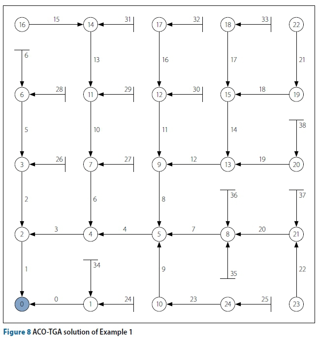
The layout of the final best solution obtained for each example problem is included. Flow directions of the pipes are shown with arrows. Adjacency nodes are indicated by straight lines at the end of a pipe. The numbers are identities assigned during the optimisation to the elements. Example 3's solutions contours are not shown for each solution.
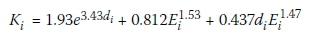
Example Network 1
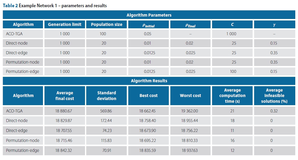
The first example network, shown in Figure 6, is a small network on a flat surface.
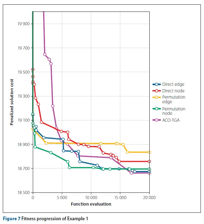
The main purpose of this example problem is to demonstrate that all algorithms are performing correctly and comparably when the space for heuristic influences is minimal. Table 2 shows the algorithm parameters used during analysis and averaged results for this network. Figure 7 shows the fitness progress with function evaluations of the best result produced by each of the five algorithms. The node strategies have slower computation time than their edge counter parts, as is expected due to the additional target-node decision required by these algorithms. The ACO-TGA has the slowest computation time of all, if only slightly worse than the node algorithms for such a small problem. On average the algorithms perform very similarly, while the node strategies and ACO-TGA are less consistent in their final results. The permutation edge approach had the worst final best solution of all the algorithms. While the ACO-TGA did find the overall best solution, it is only 0.05% better than its nearest competitor. It also had the worst overall final solution. Even for such a small example fitness warping is present in the ACO-TGA, as on average 0.32% of its total solutions were infeasible designs due to poor diameter selections. Figure 8 refers.
Example Network 2
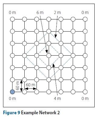
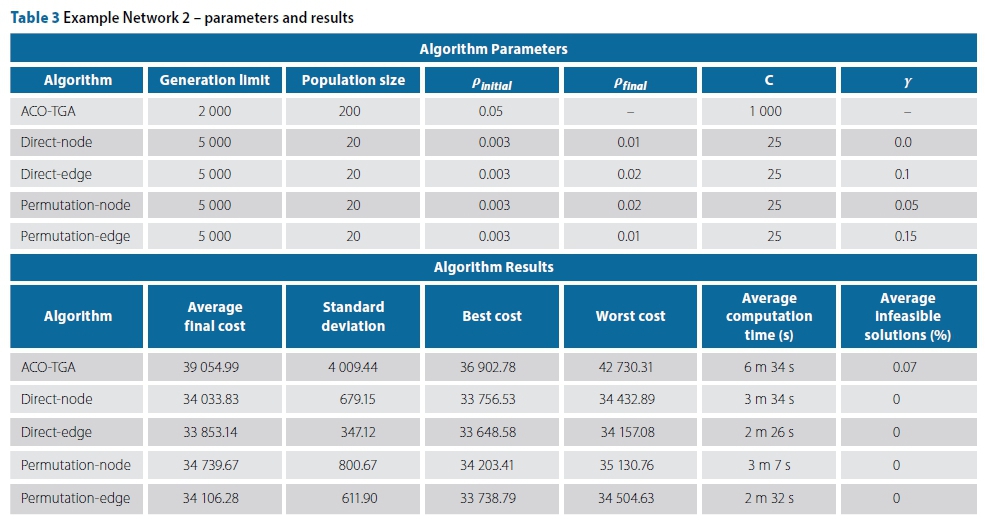
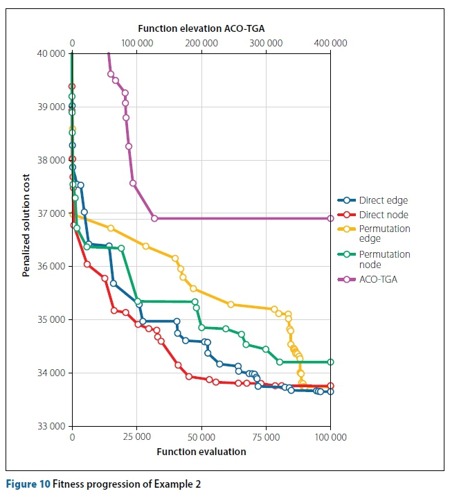
The second example, shown in Figure 9, is a medium-size network. The elevation topology mimics a hill with a flat surrounding area. The algorithm parameters during analysis and averaged results for Example Problem 2 are shown in Table 3.
The ACO-TGA performs significantly worse on average, and in its best run, than the other algorithms, while having four times as many function evaluations. It is also far less consistent. The ACO-TGA is again the only algorithm to produce infeasible solutions. On average the direct-edge strategy performs the best, while the three other newly proposed algorithms show comparable average performance. The overall best solution was found by the direct edge-strategy, while the best solution obtained by the ACO-TGA is worse than the worst solution obtained by any of the algorithms. Again, the ACO-TGA requires the most computation and the node strategies are slightly slower than their edge counter parts. The progress of the best solutions is shown in Figure 10. The secondary X-axis shows the function evaluations for the ACO-TGA. The effect of fitness warping can be observed on the ACO-TGA, as for approximately the first 50 000 function evaluations its current solution is worse than the solutions obtained by the other algorithms within 100 function evaluations. The convergence of the ACO-TGA stagnates in this example. This is similar to the results presented by Moeini and Afshar (2012).
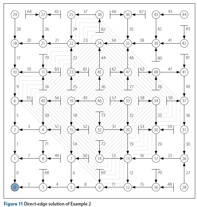
Figure 11 shows the direct-edge solution of Example 2.
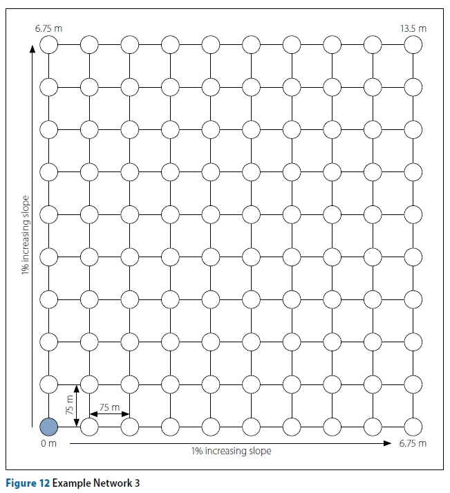
Example Network 3
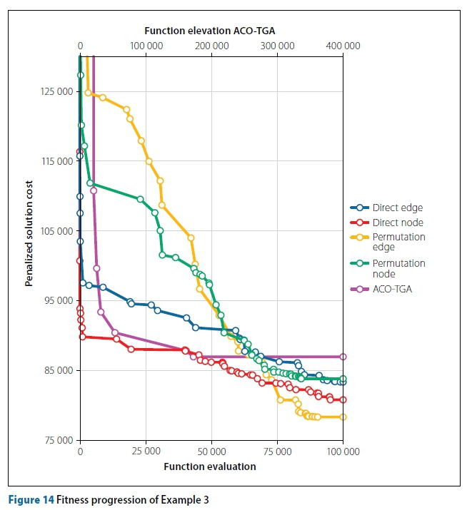
The final example, shown in Figure 12, is a large network with a gradual 1% slope. Table 4 shows the algorithm parameters and results for this example. The perm-edge algorithm performs the best of all algorithms. It obtained the best overall solution, has the best average final solution cost, and its worst solution obtained across the 20 runs is better than the best solution obtained by algorithms other than the direct-node. Fitness warping is again observed in the ACO-TGA during its early trials. The ACO-TGA performs significantly worse than the other algorithms on average and it is the most inconsistent in producing final costs. The computation time of the ACO-TGA is again the highest, while the other algorithms have comparable computation times. The rapid improvement in the ACO-TGA, whereafter it plateaus, is consistent with the results of Moeini and Afshar (2012).
Figure 13 shows the perm-edge solution of Example 3, while Figure 14 shows the fitness progression of Example 3.
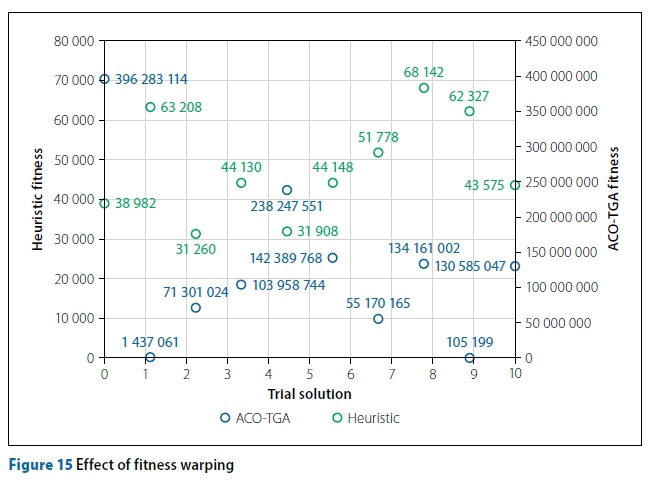
To further demonstrate the effect of fitness warping, ten trial solutions from the early stages of the ACO-TGA were randomly selected from Example Problem 1. The heuristic hydraulic optimisation algorithm of De Villiers et al (2017) was then used to perform the optimisation of the layouts of these ten trial solutions. Figure 15 shows the fitness of the ten solutions - on the left obtained by the heuristic method and on the right the fitness obtained by the ACO-TGA. The severity of the fitness warping is observed. A trial solution of the ACO-TGA with a cost of 71 303 024 produces a cost of 31 260 when the heuristic optimisation method (De Villiers et al 2017) is used to perform the hydraulic optimisation of its layout. This extreme warping of the layout's fitness due to poor diameter selections is seen in all ten cases, even for such a small example problem.
CONCLUSION
In this paper the optimisation of sewer network layout is investigated in combination with simultaneous hydraulic optimisation of the two-part sewer network design problem. Specifically, the concept of attaching a tree-growing algorithm, as proposed by Moeini and Afshar (2012), to ACO algorithms to produce feasible layouts was advanced. Four selection strategies relying on either edge-based or node-based selection were investigated. The node-based strategies require an additional decision during network construction and these decisions were resolved heuristically, but with the consequence that the network layouts that can be created are restricted. The edge-based strategies do not have this drawback and were expected to yield superior results.
Three example problems were solved using the four proposed spanning tree creation strategies as well as the original ACO-TGA proposed by Moeni and Afshar (2012) for comparison. The ACO-TGA produced, on average, the worst results for all three examples. The method used in the ACO-TGA of simultaneous layout and element size selection led to severe fitness warping in the initial trial solutions. It is difficult to say definitively that this is the only or dominant factor for the poor performance of the ACO-TGA, especially in the larger examples, but it is certainly a significant drawback which warrants caution in development of future algorithms.
For the other layout creation strategies, combined with the heuristic optimisation method of De Villiers et al (2017), performance depended on the example in question and no clear winner emerged. The edge-strategies, while not always the best option, consistently produced results at least comparable to the best strategy for all examples, making them attractive options. The most important outcome of the results is the importance of the effects the minor changes in selection strategy had on the final result. The permutation-edge strategy performed significantly better than any other for the large example problem, while performing the worst for the small problem. This can only be ascribed to the heuristic differences in the algorithms and makes a strong case for further investigation into alternative heuristics, specifically specialised heuristics coupled to terrain topology and problem size. It is recommended that at this stage no method be discarded from the investigation and, where possible, further alternatives be developed. This is due to the observed importance of heuristics and the ability to apply different heuristics to different selection strategies, which may lead to significantly improved results.
Although no clear indicator as to which selection strategy is more effective has been found in this study, the results have offered valuable insight into network optimisation in general, and indicate that further investigation into sewer network layout optimisation is warranted. Further, it has been demonstrated that the strategy where a single algorithm is used for both layout and element size selection simultaneously leads to fitness warping of early trial solutions. The set of eligible element sizes could be limited in an intelligent way, for example using the diameters of the heuristic method of De Villiers et al (2017) to reduce eligible diameter sizes to those around the size obtained heuristically, to reduce the severity of the fitness warping in, especially but not limited to, the early trial solutions. The alternative approach (of using a separate algorithm for each sub-problem) does not suffer from this drawback and should, if the challenge of computational efficiency can be overcome as with the proposed hybrid algorithms presented in this article, be favoured in future work.
REFERENCES
Afshar, M H, Shahidi, M, Rohani, M & Sargolzaei, M 2011. Application of cellular automata to sewer network optimization problems. Scientia Iranica A, 18(3): 304-312. [ Links ]
Bau, Y, Ho, C & Ewe, H 2008. Ant colony optimization approaches to the degree-constrained minimum spanning tree problem. Journal of Information Science and Engineering, 24: 1081-1094. [ Links ]
Bui, T N & Zrncic, C M 2006. An ant-based algorithm for finding degree-constrained minimum spanning tree. Computer Science Program. Middletown, PA: Pennsylvania State University at Harrisburg. [ Links ]
De Villiers, N, Van Rooyen, G C & Middendorf, M 2017. Sewer network design: Heuristic algorithm for hydraulic optimization. Journal of the South African Institution of Civil Engineering, 59(3): 48-56. [ Links ]
Diogo, A F, Walters, G A, Sousa, E R & Graveto, V M 2000. Three-dimensional optimization of urban drainage systems. Computer-Aided Civil and Infrastructure Engineering, 15(6): 409-426. [ Links ]
Diogo, A & Graveto, V 2006. Optimal layout of sewer systems: A deterministic versus a stochastic model. Journal of Hydraulic Engineering, 132(9): 927-943. [ Links ]
Dorigo, M & Stützle, T 2004. Ant Colony Optimization. Cambridge, MA: MIT Press. [ Links ]
Dorigo, M, Maniezzo, V & Colorni, A 1996. Ant system: Optimization by a colony of cooperating agents. IEEE Transactions on Systems, Man, and Cybernetics, Part B, 26(1): 29-41. [ Links ]
Haghighi, A & Bakhshipour, A E 2012. Optimization of sewer networks using an adaptive genetic algorithm. Water Resources Management, 26(12): 3441-3456. [ Links ]
Haghighi, A 2013. Loop-by-loop cutting algorithm to generate layouts for urban drainage systems. Journal of Water Resources Planning and Management, 139(6): 693-703. [ Links ]
Haghighi, A & Bakhshipour, A 2015. Deterministic integrated optimization model for sewage collection networks using Tabu Search. Journal of Water Resources Planning and Management, 141(1): 0401404. [ Links ]
Lejano, R P 2006. Optimizing the layout and design of branched pipeline water distribution systems. Irrigation and Drainage Systems, 20: 125-137. [ Links ]
Li, G & Matthew, R 1990. New approach for optimization of urban drainage systems. Journal of Environmental Engineering, 116(5): 927-944. [ Links ]
Merkle, D, Middendorf, M & Schmeck, H 2002. Ant colony optimization for resource-constrained project scheduling. IEEE Transactions on Evolutionary Computation, 6(4): 333-346. [ Links ]
Moeini, R & Afshar, M H 2012. Layout and size optimization of sanitary sewer network using intelligent ants. Advances in Engineering Software, 51: 49-62. [ Links ]
Pan, T & Kao, J 2009. GA-QP model to optimize sewer system design. Journal of Environmental Engineering, 135(1): 17-24. [ Links ]
Walters, G A 1985. The design of the optimal layout for a sewer network. Engineering Optimization, 9(1): 37-50. [ Links ]
 Correspondence:
N de Villiers
Department of Civil Engineering, Stellenbosch University
Private Bag X1, Matieland 7602
South Africa.
T: +27 83 609 9323
E: ndevilliers@lulabuild.com
E: ndv@sun.ac.za
G C van Rooyen
Department of Civil Engineering, Stellenbosch University
Private Bag X1, Matieland 7602
South Africa.
T: +27 21 808 4437
E: gcvr@sun.ac.za
M Middendorf
Department of Mathematics and Computer Science University of Leipzig
Postfach 10 09 20, D-04009 Leipzig
Germany
T: +49 341 97 32275
E: middendorf@informatik.uni-leipzig.de

DR NICO-BEN DE VILLIERS obtained a degree in Civil Engineering in 2011 from Stellenbosch University, and Immediately commenced postgraduate studies in Civil Engineering Informatics at the same Institute, In 2018 obtaining a PhD focused on sewer network design and analysis. Hels the Head of Software of Convlrt (Pty) Ltd, a software company specialising in cloud-based engineering and construction management solutions for the global market.

DrGCvan Rooyen studied science and engineering at the Universities of the Orange Free State, Pretoria and Stellenbosch, obtaining a PhD from the latter. He is currently responsible for Civil Engineering Informatics in the Department of Civil Engineering at Stellenbosch University. Before joining the lecturing staff at Stellenbosch in 1992 he worked as construction engineer for the Department of Water Affairs, and as researcher at the Institute for Structural Engineering and the Bureau of Mechanical Engineering at Stellenbosch University.

PROF DR MARTIN MIDDENDORF received the Diploma degree in Mathematics and the Dr. rer. nat. degree from the University of Hannover, Germany, in 1988 and 1992 respectively, and the Professorial Habilitation degree from the University of Karlsruhe, Germany, in 1998. He has worked at the University of Dortmund and the University of Hannover as Visiting Professor, and was Professor at the Catholic University of Eichstätt. He is currently Professor of Swarm Intelligence and Complex Systems at the Leipzig University, Germany. His research interests include swarm intelligence, algorithms from nature, optimisation and bioinformatics.

