


Services on Demand
Article
 English (pdf)
 Article in xml format
 Article references
Indicators

Related links
-
 Cited by Google
 -
 Similars in Google
Share

 Permalink
Journal of the South African Institution of Civil Engineering
On-line version ISSN 2309-8775
Print version ISSN 1021-2019
J. S. Afr. Inst. Civ. Eng. vol.59 n.3 Midrand Sep. 2017
http://dx.doi.org/10.17159/2309-8775/2017/v59n3a6
TECHNICAL PAPER
Sewer network design: Heuristic algorithm for hydraulic optimisation
N de Villiers; G C van Rooyen; M Middendorf
ABSTRACT
For a given sewer network layout and choice of pipe material, the total installed cost of the network is determined mainly by the pipe diameters and slopes. Hydraulic design optimisation is the task of determining suitable pipe diameters and slopes so as to minimise the installed cost of the network. This is a complex problem for which numerous solution approaches have been proposed. Recently the use of metaheuristic algorithms, like Ant Colony Optimisation (ACO) for example, has gained popularity, and they perform well for a given static layout. However, their computational complexity precludes their use in simultaneous layout and hydraulic optimisation, where a complete hydraulic optimisation has to be performed for each layout. This paper proposes a computationally efficient method for near optimal hydraulic design of a gravity sewer network. It makes use of required minimum slope information to heuristically determine optimal pipe sizes and slopes. The method is used to solve two benchmark problems and is shown to obtain good solutions while being computationally extremely efficient. Therefore it is ideally suited to be used in combination with a metaheuristic algorithm aimed at optimising the network layout.
Keywords: gravity sewer network, heuristic optimisation, hydraulic optimisation, contributor hydrograph, pipe size and slope
INTRODUCTION
Sewer networks form a vital part of public health in urban areas and constitute one of the most capital-intensive infrastructure investments (Wirhadikusumah et al 2001). Consequently the ability to improve sewer network designs through the use of metaheuristic optimisation algorithms could potentially yield a significant reduction in capital expenditure. Simultaneous sewer network layout and hydraulic design optimisation using these algorithms has been investigated in recent times. However, the algorithms are computationally very expensive, since the optimisation procedure responsible for the hydraulic design has to be completed for a very large number of layout attempts. Lejano (2006) found that, due to the complexity of simultaneous optimisation algorithms, most research has been done on the hydraulic optimisation sub-problem, while the layout remains static. This paper focuses on the development of a computationally efficient heuristic optimisation algorithm by which, for a given layout, all constraints of the hydraulic design are systematically satisfied using slope information. The method is applied to two benchmark problems in the literature and shown to obtain near optimal hydraulic designs, while requiring very little computational effort. These characteristics make it ideal for combination with a metaheuristic algorithm for optimal layout creation.
OPTIMISATION CONSTRAINTS AND ANALYSIS
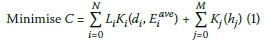
Sewer networks comprise manholes connected by sewer pipes and other components, such as pumping stations and rising mains. The network is used to collect waste water from various facilities, such as houses, schools and industrial buildings, and convey it to a sewage processing plant where the waste water is purified. The design is to be optimised, in this paper, in terms of capital investment cost. The objective function for the optimisation of simultaneous sewer network layout and hydraulic design optimisation is as per Equation 1 (Moeini & Afshar 2012), while Figure 1 shows the definition of depth variables.

Where:
C = cost function of sewer network
Li= length of pipe i, i ε {1, ... , N}
Ki= unit cost function of pipe i defined in terms of its diameter (d) and average cover depth (Eiave)
Kj= unit cost function of manhole j, defined in terms of its height (hj)
N = number of pipes in the network
M = number of manholes in the network
Sewer network design is subject to a multitude of constraints of varying complexity, as described below.
1. Cover depth
Both minimum and maximum cover depth constraints are enforced. Minimum cover depths protect pipes from imposed loads, such as vehicle loads where sewer pipes pass under roads. The minimum cover depth also prevents cross-contamination between water distribution networks by ensuring that sewer pipes are placed below water mains. Furthermore, the minimum cover depth ensures an adequate drop for house connections. Similarly, the maximum cover depth prevents pipe failure under excessive soil and imposed loads. Maximum cover depth may also be enforced to avoid excessive excavation, specifically where soil conditions are adverse.
2. Velocity
Both minimum and maximum velocity constraints are enforced at the peak design flow rate. The minimum velocity prevents the deposition of solid particles. The maximum flow velocity is enforced to prevent erosion of the pipe material.
3. Slope
A minimum slope is enforced on all pipes. This is to prevent inaccurate placement during construction, or adverse slopes resulting from pipe settlement. The minimum slope requirement also ensures that, during full-flow conditions, the minimum flow velocity is achieved.
4. Required spare capacity
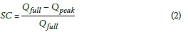
A percentage spare capacity is enforced at peak-flow conditions to ensure that pressurised flow does not occur. The constraint has the additional benefit of providing a margin of safety if storm water ingress is experienced during peak-flow times. Some investigators (Moeini & Afshar 2012; Haghighi & Bakhshipour 2015) use a maximum relative flow-depth constraint rather than percentage spare capacity. This is merely a different formulation of the same constraint. Moeini and Afshar (2012) enforce a minimum relative flow depth. In this implementation no such constraint, or an equivalent, is enforced. This constraint is not common engineering practice; furthermore, near the sources of the network it becomes almost impossible to enforce this constraint, due to unavoidable low-flow rates.
Where:
SC = spare capacity ratio
Qfull= full-flow rate (m3/s)
Qpeak= partially full-flow rate at peak conditions (m3/s)
This constraint results in partially full-flow conditions in all pipes; to solve for the hydraulic parameters, Manning's equation is used to estimate velocities throughout this investigation.
5. commercially available diameters
Diameters may only be selected from a discrete set of commercially manufactured diameters.
6. Progressive pipe diameters
The diameter of a pipe may only be equal to or larger than any of the pipes directly preceding itself. This is to prevent possible blockage, damming of waste water and sudden increase in flow velocities in the network.
7. Progressive pipe depths
The outflow pipe of any manhole may not be placed above the deepest inflow pipe. This prevents permanent damming of waste water and solid deposition in the manhole.
Contributor Hydrograph Theory is used in this implementation for accumulated flow rate calculations, taking time delays into account. The contributing hydrograph at each node is routed down the network to the outfall manhole. Theoretically this downstream routing should be done using full hydrodynamic flow analysis. However, Stephenson and Hine (1982) have demonstrated that ordinary time-lag routing is of sufficient accuracy for sewer network design purposes.
HYDRAULIC OPTIMISATION
Hydraulic optimisation of a sewer network is one part of the two-part network optimisation problem, in which element sizes, installation depths and slopes are determined for a given layout. Due to the highly constrained nature of hydraulic optimisation and the complexity of simultaneous solution algorithms, this part has seen considerably more work than the layout optimisation problem. Mays and Wenzel (1976) applied dynamic programming (DP) to the design of gravity sewer networks with the assumption that the direction of flow is fixed, severely restricting the set of problems to which their concepts may be applied. Robinson and Labadie (1981) also applied DP to develop an optimisation procedure. Miles and Heaney (1988) developed a storm water drainage design method using a spreadsheet package which may be applied to static layouts. More recently non-classic optimisation algorithms have been developed. Diogo and Graveto (2006) developed a comprehensive enumeration model and simulated annealing (SA) algorithm for the layout and component size optimisation of sewer networks. Afshar (2006; 2012) and Afshar et al (2011) have applied numerous non-classic optimisation techniques to the sewer network hydraulic design problem, namely an ant colony algorithm (ACO) (2006), cellular automata (CA) (2011), a rebirthing genetic algorithm (RGA) (2012), and more recently a hybrid genetic algorithm (GA) and general hybrid cellular automata (GHCA) were proposed for the efficient and effective optimal design of pumped sewer networks with fixed layouts (Rohani & Afshar 2015). The lack of computational efficiency of these algorithms restricts combining them with a non-classic optimisation algorithm for layout optimisation, due to the resulting computation times.
Some hydraulic optimisation algorithms have been developed and successfully combined with layout optimisation algorithms, all with different advantages and disadvantages. Walters (1985) used DP for simultaneous layout and size optimisation, and his method could be used to drain a set of sources with fixed positions. Li and Matthew (1990) used discrete differential dynamic programming (DDDP), which utilised an iterative procedure to generate the layout, and then to size the sewers and pumps while keeping the layout fixed. DDDP has some significant drawbacks - it restricts the search space and reduces the probability of locating the global optimum. The DDDP stages must be manually divided for each individual problem and this reduces its practicality. Pan and Kao (2009) used a genetic algorithm (GA) combined with quadratic programming (QP). In their approach a majority of the constraints were formulated in QP, while other parameters, such as layout and pipe diameters, were determined by the GA. Moeini and Afshar (2012) proposed an ant colony optimisation (ACO) algorithm, combined with a tree growing (TG) algorithm, which performs both the layout construction and selects diameters simultaneously. In their approach an assumption of sewer flow at maximum relative depth is made, allowing for the calculation of pipe slopes. Haghighi and Bakhshipour (2015) combined previous works, namely the loop-by-loop cutting algorithm (Haghighi 2013) and an adaptive genetic algorithm (Haghighi & Bakhshipour 2012), with a tabu search (TS) algorithm to create an effective hybrid algorithm for simultaneous layout and element size optimisation.
The approach followed by both Moeini and Afshar (2012), and Pan and Kao (2009) to use a single selection algorithm for both layout and element sizing has the advantage of computational efficiency while suffering from what will be termed here as fitness warping. With this approach a layout is constructed, and simultaneously element sizes (in this case diameter of pipes) are selected. In the initial iterations of an evolutionary optimisation algorithm the population often comprises entirely randomly selected solutions. It is therefore unlikely that good solutions have been found, or that the algorithm has started to converge around a good or optimal region in the search space for either sub-problem. If the algorithm produced a very good layout during, especially, but not limited to, its early iterations it is very unlikely that the accompanying diameters will also fall within a very good region of the search space. The result is that the overall fitness of the solution is poor, due to the poor diameter selection, despite the very good layout. Consequently, the algorithm is unable to recognise that a good layout has been found. To overcome this drawback, a hydraulic optimisation procedure is required which is well suited to be combined with an algorithm responsible only for layout construction. It must be able to compute all hydraulic design parameters. To this end a new heuristic optimisation algorithm is proposed, which uses a systematic iterative approach to select diameters while satisfying all hydraulic design constraints. The algorithm operates under the heuristic that increasing diameters, in order to reduce the required slope by a significant margin, leads to economic decisions. The algorithm relies entirely on this heuristic to obtain near-optimal costs. The cost of the final design is only calculated once the entire design has been completed. The mathematical derivations, formulae and engineering concepts relevant during the heuristic procedure are described hereafter.
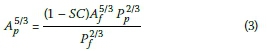
Referring to constraint 4 above (under Optimisation Constraints and Analysis), Manning's equation for partially full-flow conditions is used. From Manning's equation it is clear that flow rate, diameter and slope are interdependent variables. As described earlier, the accumulated flow rates are dependent on network layout. The diameter selections are limited to a set of commercially available diameters, while the slope is a continuous variable with an upper and lower bound. Once flow rates and diameters are known, the required slope can be calculated directly to satisfy Manning's equation, i.e. partially full flow that provides the required spare capacity of constraint 4. Substituting Manning's equation into Equation 2, and after some manipulation, yields:
Where:
Ap = partial-flow area (m2)
SC = spare capacity ratio
Af = full-flow area (m2)
Pp = partially wetted perimeter (m)
Pf = wetted perimeter at full flow (m)
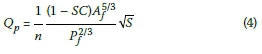
Substituting this into Manning's equation for partial-flow conditions, Qp, after some manipulation, yields:
Where:
Qp= flow rate at partial-flow conditions (m3/s)
S = slope of the pipe (m/m)
n = Manning Roughness Coefficient
All other variables are as defined in Equation 3.
Equation 4 ensures that the conditions of constraint 4 are satisfied if used to calculate the slope, while additionally allowing for the calculation of slopes in terms of the full-flow area and wetted perimeter. Constraint 6 (progressive pipe diameters) can be directly enforced during the diameter selection process. This is done by selecting diameters in sequence, ensuring that all upstream pipes of the current pipe already have their diameters selected, and adjusting the lower-bound of the set of eligible diameters for the current pipe accordingly.
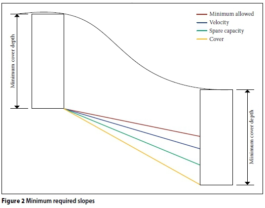
The lower-bounding slope of a pipe is influenced by a number of constraints, as indicated in Figure 2. All of the constraints have to be satisfied simultaneously, as described below.
Minimum required slope
This value is specified.
Minimum allowable cover depth
Cover depth requirements may enforce a steep slope on pipes in order to achieve the necessary depth at the downstream manhole, as shown in Figure 2.
Minimum velocity
The minimum velocity constraint, combined with Manning's equation, yields:
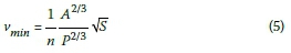
As vminis a known constant, the flow area, A, and wetted perimeter, P, can be determined if the flow depth can be determined. Then the required slope, S, to achieve the required minimum velocity, can be calculated.
The flow depth can be calculated using the hydraulic equation Q = vA. The flow rate is known if the calculation is carried out in a topological sort order, as described further on. The only unknown remaining is the partial-flow area, as v is substituted for vminor vmaxdepending on the slope being calculated. Rewriting the hydraulic equation to allow solving with a line search algorithm yields:

Equation 6 is obviously a minimum when Q = vA; in all other cases a value > 0 is obtained. It should also be noted that it is important to solve for the flow depth and not just the area, as in Equation 5 the wetted perimeter is also required. The flow area and wetted perimeter may be written in terms of the flow depth (also refer to Figure 3).
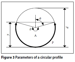
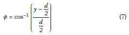
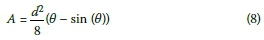
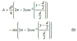
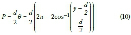
Substituting the expressions for the area in terms of the flow depth into Equation 6 yields a highly implicit equation in terms of both the diameter and flow depth. Diameters are selected beforehand, so the flow depth can be solved for using a line search algorithm. In this implementation an interval-halving algorithm is used. Once the flow depth is known, it is used in Equation 5 to solve for the minimum required slope to achieve the minimum allowed velocity. Increasing the slope increases the flow velocity. It should be noted that in all equations of this section vmincould be substituted for vmax, or any other known velocity, to obtain the required slope to achieve the specified velocity.
Required spare capacity
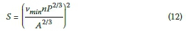
The required spare capacity constraint also allows for the calculation of a minimum required slope. Increasing the slope above this minimum value does not violate the constraint. Using Equation 4 the required slope can be calculated in terms of the flow area and wetted perimeter. The only design parameter required to calculate these values is the diameter, which at this stage is known. Using Equations 2 and Manning's equation, an expression for the required slope is found:
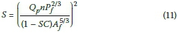
Where:
S = required slope to achieve minimum spare capacity (m/m)
Qp= flow rate at partial-flow conditions (m3/s)
n = Manning roughness coefficient
 = wetter perimeter at full flow (m)
SC = spare capacity ratio
 = full-flow area (m2)
After accounting for all the lower-bounding slope constraints, the next step is to determine when increasing the diameter is potentially beneficial, i.e. when an increment in diameter leads to a reduction in slope and consequently an expected reduction in cost. For the first two cases, namely minimum allowable slope and cover requirements, increasing the diameter obviously has no effect on the required slope. In the other cases, namely velocity and spare capacity, increasing the diameter may prove to be beneficial. This is tested by keeping the flow rate and Manning roughness constant, and varying the diameter while calculating required slopes. Using Q = 15 ℓ/s, n = 0.015, v = 0.75 m/s and SC = 0.3, the required slopes for various diameters are shown in Figure 4.
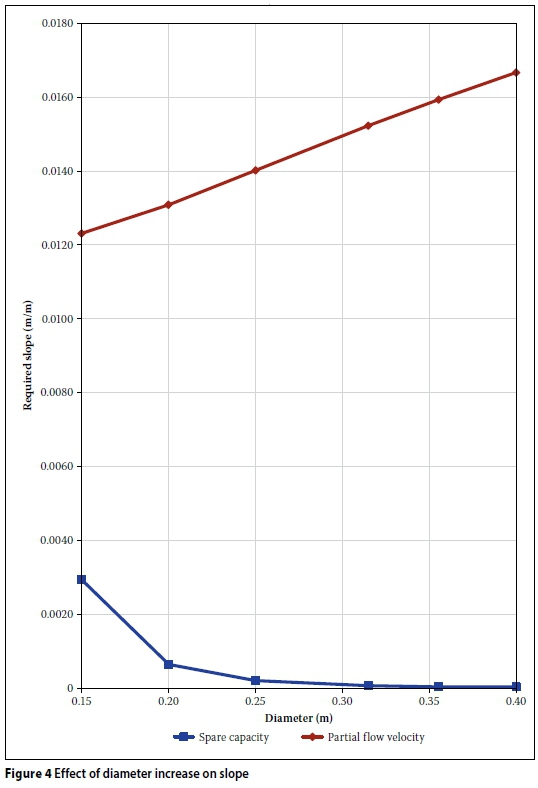
Figure 4 (p 51) shows that increasing the diameter affects the required slopes differently. The required slope to maintain a minimum spare capacity decreases, while the required slope to achieve a specified velocity increases. This increase in slope for velocity is counter to what is common in engineering practice. When Equation 5 is used to calculate the required slope, the assumption of full-flow conditions is often made. If the assumption of full-flow conditions is made, then increasing the diameter reduces the required slope to achieve the minimum velocity. Using the hydraulic equation Q = vA, if both the flow rate, Q, and the velocity, v, remain constant, then the flow area, A, also remains constant. When assuming full-flow conditions under the same minimum velocity for a larger diameter, the flow area increases and consequently so does the flow rate. It is due to this increase in flow rate and flow area that the required slope decreases. In the case of Figure 4, the flow rate and velocity are kept constant, and consequently so is the flow area. When the diameter increases, the flow area is maintained by a decrease in flow depth. This increase in diameter leads to an increase in wetted perimeter, despite the reduction in flow depth. Referring again to Equation 5, rewriting in terms of the slope yields:
All the variables in this equation remain constant during a diameter increment, apart from wetted perimeter, P, which increases. As P is directly proportional to the slope, S, this leads to an increase in the required slope.
This implies that increasing the diameter may be beneficial in two cases: (i) when spare capacity is the active lower-bound slope constraint, and (ii) when maximum velocity is the active upper-bound slope constraint. These possibilities should be evaluated before accepting any diameter increase as beneficial. Consequently the change in slope is evaluated by parameter γ:
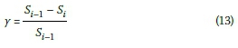
Where:
γ = slope change factor
Si= required slope for the current diameter (m/m)
Si-1 = required slope for the previous diameter (m/m)
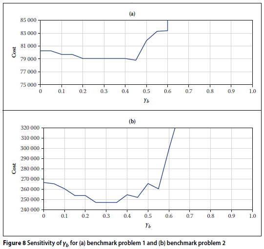
If γ > γb, where 0.0 < γb< 1.0, the increase in diameter is considered beneficial, i.e. the diameter increment leads to a sufficient enough reduction in slope that a reduction in capital expenditure can be expected. Otherwise the previous diameter is accepted if it resulted in a feasible design. If the current diameter is the first eligible diameter, this evaluation step is simply skipped. γb, the beneficial slope change factor, is a predefined variable of the optimisation procedure, similar to the evaporation rate of ACO or the mutation rate of a GA, which must be calibrated for a specific problem. γb is best understood by evaluating the effects of its extreme values on the final solution. At γb= 0 any reduction in slope is always considered beneficial, i.e. the least buried depth solution is obtained. At γb= 1 the steepest feasible slope is used, as no reduction in slope is ever considered beneficial, i.e. the smallest diameter which results in a feasible slope is used for each pipe. In most cases this results in capacity being the active minimum slope constraint. This is similar to the assumption Moeini and Afshar (2012) make in their hydraulic analysis procedure, where the flow depth is assumed to always be the maximum allowable. However, their diameter is not necessarily the smallest feasible. Li and Matthew (1990) found in their work that a balance between minimum buried depth and other feasible slopes resulted in better results than either extreme. The optimisation procedure should be repeated for multiple values of γbto determine the best value. Figure 8 (p 56) shows a sensitivity analysis of the γb parameter for the two benchmark problems discussed further on (under Results).

In all cases when determining the required slopes from hydraulic parameters, the peak design flow rate is required. The accumulated flow rates, calculated with contributor hydrograph theory, are not only dependent on the network layout, but also the network elements, as time delay is considered. This problem is addressed by performing the hydraulic design of the network in the topological sort order of the layout graph, which can always be found, as only gravity sewer networks with no cycles are considered. Inflow hydrographs are defined at all manholes, thus the flow rate of the outgoing pipe of any manhole with no inflow pipes is immediately known. Starting the design from these manholes, the hydraulic design and placement of the outgoing pipe can be completed using the equations described in this section. The hydrograph of this outgoing pipe can then be added to the hydrograph of the target manhole, with time delay included, since all the required hydraulic parameters have been determined. This procedure is continued downstream until all network components have been designed. Determining the topological sort order can be combined with the design procedure. In the topological sorting algorithm, vertices with no incoming edges are placed first, thereafter vertices are only added once all their preceding vertices have been included in the ordering. In this case manholes may be added if they have no incoming pipes, or if the hydraulic design of all its incoming pipes has been completed. Manhole depths are set to the maximum excavation depth of all incoming pipes.
Some rare special cases may be encountered during the procedure, which compromise the feasibility of the design. The special cases, listed below, are dealt with as described:
i. The minimum allowable slope exceeds the maximum allowable velocity slope:
The diameter must be increased to restore feasibility.
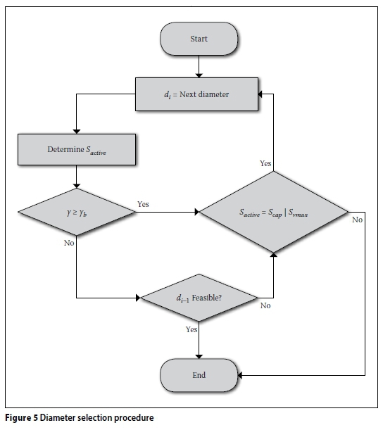
ii. The slope is dictated by minimum cover: The active slope constraint is cover, and is exceeding the maximum allowable velocity slope. Increasing the diameter would increase the maximum allowable velocity slope to restore feasibility. Alternatively, it is possible to increase the upstream depth of both the pipe and manhole to accommodate the required slope. This decision is again evaluated by γ. It is possible that this increased cover depth may exceed the maximum allowable cover depth, in which case increasing the diameter is the only option to restore feasibility. Figure 5 shows a simplified flow chart of the pipe diameter selection procedure. This procedure is repeated for all pipes, as described above, in the topological sort order of the layout.
Where:
D = the eligible set of diameters, satisfying constraints 5 and 6, in ascending order
di= the current diameter in D
di-1= the previous diameter in D
Sactive= the active, or critical, minimum slope
Scap= required slope to achieve spare capacity
Svmax= required slope to achieve maximum velocity
γ = slope change factor
γb= beneficial slope change factor
Referring to Figure 5, the procedure starts by selecting the smallest eligible diameter in D, and is then incremented by one with each iteration. The minimum required slopes for cover, minimum and maximum velocity, and spare capacity are calculated as described in this section. The largest of all the minimum slopes, including minimum required, is selected as the active, or critical, minimum slope, Sactive. If diis not the smallest diameter in D, then previous slope information is available and γ is calculated using Equation 13. If it is the smallest diameter, the evaluation of Y is simply skipped at this iteration. If γ > γbthe change in diameter is considered beneficial, i.e. the reduction in slope is expected to reduce the cost. If the change in diameter is considered beneficial, it may be possible that further increments are also beneficial. If the active slope is either the spare capacity, Scap, or maximum velocity, Svmax, another diameter increment is applied and the procedure restarted. If neither was the active slope, the current diameter is accepted. If no diameter increment was possible the current diameter is accepted and the maximum velocity slope prioritised over spare capacity. Where the diameter increment is not considered beneficial, γ < γb, the previous diameter is checked for feasibility.
If the previous diameter resulted in a feasible slope, it is accepted as the diameter for the pipe. If it did not, the active slope constraints are checked to determine if a diameter increment may be beneficial.
Once a pipe has its diameter and slope calculated, using the procedure above, the upstream hydrograph of the pipe is routed downstream, with time-delay, and added to the cumulative flow rate in the downstream manhole. This procedure is continued downstream until all pipes have had their slope and diameter calculated. Once the entire design of the network is completed, the cost function, Equation 1, is used to determine the total cost of the design.
RESULTS
Two benchmark problems are used to determine the effectiveness of the heuristic diameter selection algorithm. In both cases a maximum relative flow depth and static flow values are specified. In order to ensure the proposed heuristic procedure is accurately compared to the preceding algorithms, the relative flow depth of the result cannot exceed the specified value. The maximum relative flow-depth parameter is never directly incorporated. The spare capacity is set to a value which results in a maximum relative flow depth very close to, but still below, the specified maximum. The static flow rates are incorporated by simply disabling the downstream routing of flow rates during the optimisation of the benchmark problems to allow direct comparison of results.
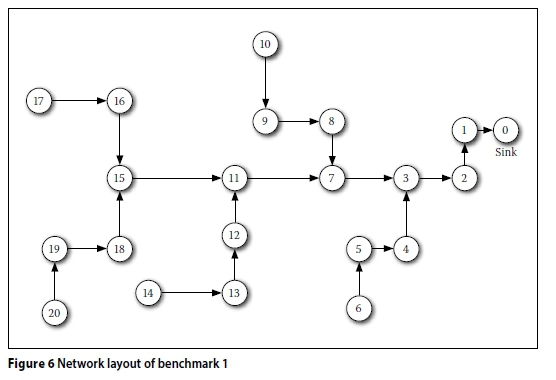
The first example is a network originally designed by Mays and Wenzel (1976), which has since been solved by other investigators. The network, shown in Figure 6, has 21 manholes and 20 pipes. The unit cost functions of Equation 1 proposed for this problem is (Meredith 1972):
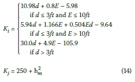
Where:
d = the diameter of pipe i ( ft)
E = the average cover depth of pipe i ( ft)
hm= the height of manhole m ( ft)
The pipe unit cost, Ki, is obtained in $/ft and the manhole unit cost, Kj, in $. The Manning coefficient for all pipes is taken as 0.013. The maximum allowable relative flow depth, ( ), is taken as 0.82. The minimum allowable cover depth, Emin, is taken as 2.4 m. The minimum velocity, vmin, and maximum velocity, vmax, is taken as 0.6 m/s and 3.6 m/s respectively. The minimum allowable slope is 0.001 (m/m). The set of commercially available pipes {D} = {304.8 mm (12 in), 381 mm (15 in), 457.2 mm (18 in), 533.4 mm (21 in), 762 mm (30 in), 914.4 mm (36 in), 1 066.8 mm (42 in), 1 219.2 mm (48 in)}. Table 1 shows the necessary data for the benchmark problem.
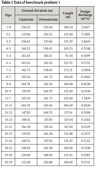
Table 2 shows the results obtained by various methods for the problem. The proposed heuristic method is able to achieve a result similar to the metaheuristic optimisation methods, while requiring 6 milliseconds of computation time using a personal computer with 3rd generation Intel Core i7-3630QM.

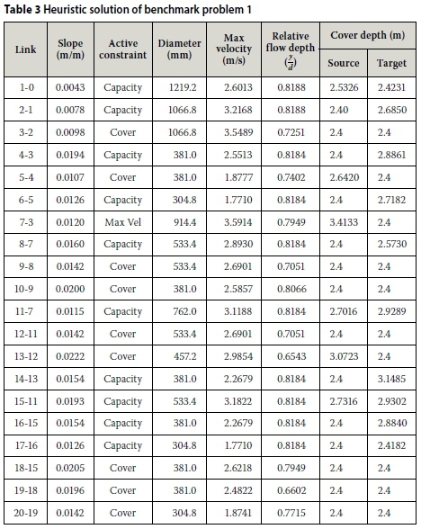
Table 3 shows the detailed solution obtained by the proposed heuristic method. Table 3 indicates the method's ability to differentiate between the benefit of minimum possible slopes and diameter increments. Note that for pipe 7-3 the special case where the cover slope exceeds the maximum allowable velocity slope is encountered. The cover depth of the pipe at the source end and the depth of its source manhole are increased to achieve the required slope.
The second problem, shown in Figure 7, is part of the "Kerman" network in Iran (Afshar et al 2011). For this example the unit cost functions given in Equation 15 (Afshar et al 2011) are used in conjunction with Equation 1 for cost calculations.
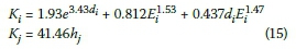
Where:
di= the diameter of pipe i (m)
Ei= the average cover depth of pipe i (m)
hj= the height of manhole j (m)
The Manning coefficient for all pipes is considered as 0.013. The maximum allowable relative flow depth, ( ), is considered as 0.82. The minimum allowable cover depth, Emin, is considered as 2.45 m. The minimum velocity, vmin, and maximum velocity, vmax, are considered as 0.3 m/s and 3.0 m/s respectively. The minimum allowable slope is 0.001 (m/m). The set of commercially available pipes, {D} = {150 mm, 200 mm, 250 mm, 300 mm, 400 mm, 500 mm, 600 mm, 700 mm}.
The necessary data for the definition of benchmark problem 2 is shown in Table 4. The problem is solved using the proposed heuristic method. Table 5 shows the results obtained by various methods while solving the problem. All values shown in Table 5, except for the newly proposed heuristic method, were presented by Afshar et al (2011).
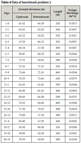
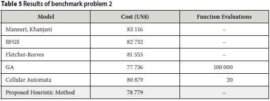
Table 5 shows the algorithm's ability to obtain a near-optimal solution while also only requiring 6 milliseconds of computation time. Table 6 shows the detailed solution produced by the heuristic method for benchmark problem 2.
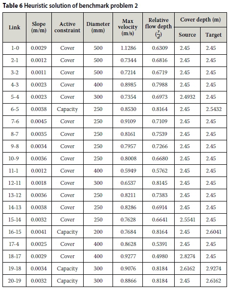
Figure 8 shows a sensitivity analysis of the γb parameter for both problems. From this figure it is clear that the value of γbis not very sensitive to small changes around the optimum. However, some improvement in the final cost is gained from repeating the algorithm for multiple values of γb. Because γbis not sensitive around the optimum, it may be calibrated where multiple similar networks have to be optimised. This avoids having to repeat the solution of each problem multiple times for each problem. However, the algorithm is computationally efficient enough that repetitions do not inhibit its usability, even when combined with a computationally expensive layout optimisation algorithm.
From these benchmark problems it becomes clear that the heuristic algorithm maintains near-optimal solution quality while having almost instantaneous computation time. This makes it ideally suited for combining with an ACO or similar algorithm responsible for layout creation that requires a significant amount of function evaluations (100 000+), each of which requires a hydraulic optimisation run.
CONCLUSION
In this paper a heuristic optimisation algorithm, which relies on the assumption that keeping slopes to a relative minimum while increasing diameters leads to economic decisions, was proposed. The algorithm solves the problem incrementally, determining the hydraulic parameters of each element individually. The algorithm was applied to two previously proposed benchmark problems and was shown to be able to produce near-optimal results with very little computational effort. The results obtained by this algorithm, due to its computational efficiency and solution quality, can be used to seed the set of eligible hydraulic parameters of other, more computationally expensive, optimisation methods, reducing the size of the search space. This method is ideally suited to be combined with a non-classical, computationally expensive, optimisation algorithm which aims to optimise the network layout, as will be shown in a follow-up article by the authors. The algorithm produces static results for a static layout. This allows layout creation techniques to be compared more directly, as the fitness of a given layout is not dependent on a non-classical optimisation algorithm's varying performance.
REFERENCES
Afshar, M H 2006. Application of a max-min ant system to joint layout and size optimization of pipe networks. Engineering Optimization, 38(3): 299-317. [ Links ]
Afshar, M H, Shahidi, M, Rohani, M & Sargolzaei, M 2011. Application of cellular automata to sewer network optimization problems. Scientia Iranica, 18(3): 304-312. [ Links ]
Afshar, M H 2012. Rebirthing genetic algorithm for storm sewer network design. Scientia Iranica, 19(1): 11-19. [ Links ]
Diogo, A & Graveto, V 2006. Optimal layout of sewer systems: A deterministic versus a stochastic model. Journal of Hydraulic Engineering, 132(9): 927-943. [ Links ]
Haghighi, A & Bakhshipour, A E 2012. Optimization of sewer networks using an adaptive genetic algorithm. Water Resources Management, 26(12): 3441-3456. [ Links ]
Haghighi, A 2013. Loop-by-loop cutting algorithm to generate layouts for urban drainage systems. Journal of Water Resources Planning and Management, 139(6): 693-703. [ Links ]
Haghighi, A & Bakhshipour, A 2015. Deterministic integrated optimization model for sewage collection networks using Tabu Search. Journal of Water Resources Planning and Management, 141(1): 0401404. [ Links ]
Lejano, R P 2006. Optimizing the layout and design of branched pipeline water distribution systems. Irrigation and Drainage Systems, 20: 125-137. [ Links ]
Li, G & Matthew, R 1990. New approach for optimization of urban drainage systems. Journal of Environmental Engineering, 116(5): 927-944. [ Links ]
Mays, L W & Wenzel, H G 1976. Optimal design of multilevel branching sewer systems. Water Resources Research, 12(5): 913-917. [ Links ]
Meredith, D D 1972. Dynamic programming with case study on planning and design of urban water facilities. Treaties on urban water systems. Fort Collins, CO: Colorado State University. [ Links ]
Miles, S & Heaney, J 1988. "Better than optimal" method for designing drainage systems. Journal of Water Resources Planning and Management, 114(5): 477-499. [ Links ]
Moeini, R & Afshar, M H 2012. Layout and size optimization of sanitary sewer network using intelligent ants. Advances in Engineering Software, 51: 49-62. [ Links ]
Pan, T & Kao, J 2009. GA-QP model to optimize sewer system design. Journal of Environmental Engineering, 135(1): 17-24. [ Links ]
Robinson, D K & Labadie, J W 1981. Optimal design of urban storm water drainage system. Proceedings, International Symposium on Urban Hydrology, Hydraulics, and Sediment Control. Lexington, KY, 145-156. [ Links ]
Rohani, M & Afshar, M H 2015. GA-GHCA model for the optimal design of pumped sewer networks. Canadian Journal of Civil Engineering, 42(1): 1-12. https://doi.org/10.1139/cjce-2014-0187. [ Links ]
Stephenson, D & Hine, A E 1982. Computer analysis of Johannesburg sewers. Proceedings of the Institute of Municipal Engineering of Southern Africa (IMESA), 7(4): 13-23. [ Links ]
Walters, G A 1985. The design of the optimal layout for a sewer network. Engineering Optimization, 9(1): 37-50. [ Links ]
Wirahadikusumah, R, Abraham, D & Iseley, T 2001. Challenging issues in modeling deterioration of combined sewers. Journal of Infrastructure Systems, 7(2): 77-84. [ Links ]
 Correspondence:
N de Villiers
Department of Civil Engineering
Stellenbosch University
Private Bag X1
Matieland 7602
South Africa
T: +27 83 609 9323
E: ndv@sun.ac.za
E: ndv@convirt.co.za
G C van Rooyen
Department of Civil Engineering
Stellenbosch University
Private Bag X1
Matieland 7602
South Africa
T: +27 21 808 4437
E: gcvr@sun.ac.za
M Middendorf
Department of Mathematics and Computer Science
University of Leipzig
Postfach 10 09 20
D-04009 Leipzig
Germany
T: +49 341 97 32275
E: middendorf@informatik.uni-leipzig.de

NICO-BEN DE VILLIERS obtained a degree in Civil Engineering in 2011 from Stellenbosch University, and immediately commenced postgraduate studies in Civil Engineering Informatics at the same institute. He is currently concluding his PhD, which focuses on optimisation of sewer network design. He is also the Technical Director of Convirt (Pty) Ltd, a software company specialising in engineering and construction management solutions for the global market.

DR GC VAN ROOYEN studied science and engineering at the Universities of the Orange Free State, Pretoria and Stellenbosch, holding a PhD from the latter. He is currently responsible for Civil Engineering Informatics at the Department of Civil Engineering at Stellenbosch University. Before joining the lecturing staff at Stellenbosch in 1992 he worked as construction engineer for the Department of Water Affairs, and as researcher at the Institute for Structural Engineering and the Bureau of Mechanical Engineering at Stellenbosch University.

PROF DR MARTIN MIDDENDORF received the Diploma in Mathematics and the Dr. rer. nat. degree from the University of Hannover, Germany, in 1988 and 1992, respectively, and the Professorial Habilitation degree from the University of Karlsruhe, Germany, in 1998. He has worked at the University of Dortmund and the University of Hannover as Visiting Professor, and was Professor at the Catholic University of Eichstätt. He is currently Professor of Swarm Intelligence and Complex Systems at the Leipzig University, Germany. His research interests include swarm intelligence, algorithms from nature, optimisation and bioinformatics.

