TECHNICAL PAPER

 

Seepage column hydraulic conductivity tests in the geotechnical centrifuge

 

 

W D van Tonder; S W Jacobsz

Correspondence

 

 

---

ABSTRACT

Provided that inter-particle flow remains laminar, hydraulic conductivity tests can be carried out in a centrifuge to accelerate flow, allowing the hydraulic conductivity of relatively impervious materials to be measured within a reasonable time. It is well documented that the inter-particle flow velocity in the centrifuge increases linearly with acceleration, and a debate in the literature deals with whether hydraulic conductivity also scales with acceleration or not. A number of hydraulic conductivity tests were carried out using seepage columns in the geotechnical centrifuge in which pore pressures were recorded within the samples during testing. When hydraulic conductivity is calculated from the hydrostatic potentials measured during testing, the hydraulic conductivity is found to be independent of the imposed acceleration. It is therefore advocated that the hydrostatic potential is scaled in the centrifuge rather than the hydraulic conductivity. It must therefore be recognised that the hydraulic gradient used in the conductivity calculation does not remain constant, but changes with the imposed acceleration.

Keywords: falling head, geotechnical centrifuge, hydraulic conductivity, seepage scaling laws, pore pressure transducer

---

 

 

INTRODUCTION

For modelling purposes it is often necessary to assess the hydraulic conductivity of materials from the field by means of laboratory testing. Provided that representative high-quality samples can be taken, a variety of test methods are available. These include falling and constant head hydraulic conductivity tests. Such tests on materials with a low hydraulic conductivity can be time-consuming. To reduce testing time, such tests can be carried out under elevated hydraulic gradients in the laboratory, for example in the triaxial apparatus. Another possibility to reduce testing time is to carry out the tests at elevated accelerations using a suitable centrifuge. The increased acceleration accelerates flow, allowing results to be obtained in a shorter time. However, the analysis of hydraulic conductivity test results at elevated acceleration requires careful consideration.

 

SEEPAGE FLOW THROUGH POROUS MEDIA

Seepage is the term used to describe the movement of pore water through a porous material. This flow is driven by a difference in mechanical energy, from an area of high mechanical energy towards an area of low mechanical energy. The total mechanical energy at a point is known as the hydrostatic potential (H) as expressed by Bernoulli's equation. The total hydrostatic potential per unit weight of water is the sum of the pressure head (h_p), elevation head (h_z) and velocity head (h_v). However, as natural seepage velocities are normally small enough to be ignored, the total hydrostatic potential is approximated by Equation 1.

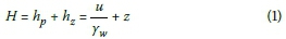
In Equation 1 u is the pore water pressure, Y_wthe unit weight of water and z the elevation of the water above a chosen datum.

The units of Equation 1 are those of length, and the hydrostatic potential is therefore conventionally expressed in metres above a chosen datum. For a saturated porous medium, when a fluid is at rest, hydrostatic conditions prevail and the hydrostatic potential will be constant at each point within the medium. In the case of zero seepage flow, the total head under hydrostatic conditions is typically taken as the elevation of the free water surface. However, for a moving fluid the hydrostatic potential varies in space and/or time (Bear 1972). Differences in the hydrostatic potential from one point to another result in a hydraulic gradient (i), resulting in seepage in the direction of decreasing potential.

Seepage flow through a fully saturated porous medium is described by Darcy's law (Equation 2), with the volumetric discharge rate (Q) a function of the hydraulic conductivity (k), the hydraulic gradient (i) and the cross-sectional through-flow area (A).

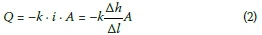
The negative symbol denotes the reducing hydrostatic potential along the flow path. The hydraulic conductivity (often also referred to by engineers as the coefficient of permeability) has units of velocity, and is a measure of the resistance of a porous medium to the flow of water. The hydraulic conductivity (k) is largely dependent on the size of the pore spaces within the porous medium. Hence, k is related to the particle size distribution, the shape of the particles and the manner in which these particles are arranged in the porous medium (structure and density), with a finer porous medium having a lower hydraulic conductivity (see for example the traditional texts by Hazen (1892) and Kozeny (1927), and more recently Alyamani and Sen (1993) and Chakraborty et al 2006)).

However, the hydraulic conductivity is as much dependent on the properties of the permeant as the properties of the porous medium. For example, temperature will have a direct effect on k as it alters the viscosity of a fluid. As demonstrated by Equation 3, k is inversely proportional to the fluid dynamic viscosity (μ) and directly proportional to K (the intrinsic permeability with units of m²) and fluid density ρ.

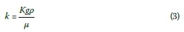
The intrinsic permeability (K) is an absolute coefficient which depends on the characteristics of the porous medium only. Hence, k will decrease with an increase in dynamic viscosity at lower temperatures.

Darcy's law requires that all flow should be laminar so that resistive viscous forces dominate at low fluid velocities (Culligan-Hensely & Savvidou 1995; Singh & Gupta 2002). When flow velocities increase, the inertial forces are sufficiently high to overcome the resistive viscous forces, and the flow is said to be turbulent. Hence, at high fluid velocities, turbulent flow dominates and Darcy's law is invalid. To determine whether flow is laminar or turbulent, four factors are considered in the calculation of the Reynolds number (Re) (Equation 4). For Darcy's law to be valid, Fetter (2001) states that the Reynolds number (Re) should be less than 1 to 10, depending on the granular medium. In most cases seepage flow in porous media is slow enough for Darcy's law to be valid, except where there are large cavities/fractures or steep hydraulic gradients (Fetter 2001).

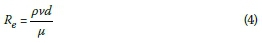
In Equation 4 v is the specific discharge velocity and d is the characteristic microscopic length of the medium (often taken as the effective particle size, typically assumed to be D₁₀ (Singh & Gupta 2000)).

Scaling laws

As with the geometry and material properties of a centrifuge model, the flow in the model needs to be representative of that in the prototype. To achieve the required similitude between the model and prototype, the flow of water needs to be properly scaled (Nakajima & Stadler 2006). As mentioned by numerous authors (e.g. Taylor 1995; Dell'Avanzi & Zornberg 2002; Thusyanthan & Madabhushi 2003; Nakajima & Stadler 2006), the primary scaling law for flow in a centrifuge is that of seepage velocity (v), as shown in Equation 5.

The seepage velocity in the centrifuge model (v_m) will be N times greater than in the prototype (v_p) it represents (Taylor 1995). As stated by Thusyanthan & Madabhushi (2003), this scaling law has been proven experimentally, provided that the prototype soil is used in the model and the soil is fully saturated (Taylor 1995).

However, when one considers Darcy's equation governing seepage flow, two opposing issues arise. The debate deliberates whether the hydraulic conductivity (k) or the hydraulic gradient (i) is the fundamental parameter affected by increased acceleration (Taylor 1995; Thusyanthan & Madabhushi 2003). Some researchers (e.g. Singh & Gupta 2000) consider hydraulic conductivity (k) to be directly proportional to acceleration, and suggest that the gradient (i) is independent of acceleration as it is dimensionless. Thus, if i is independent of acceleration, then i_m= i_pand k is a function of the acceleration imposed by the centrifuge. Based on this argument,

This results in the scaling law for seepage velocity being satisfied.

As outlined by Taylor (1995) and Thusyanthan and Madabhushi (2003) the problem with this argument is that soils would appear to be impermeable under zero gravity. This is due to the assumption of all seepage flow being gravity-driven and at zero gravity there would not be any pressure gradient to induce seepage flow through the soil (Taylor 1995).

However, based on the definition of the hydraulic gradient (Equation 2), and as stresses are equal to those of the prototype, while the lengths are condensed N times in the centrifuge, Taylor (1995) and Thusyanthan and Madabhushi (2003) proposed that the hydraulic gradient is N times larger than in the prototype. The increased acceleration results in an increase in the potential energy per unit volume of fluid. This results in the change in head (Δh) having to occur over a length N times smaller than in the prototype. Therefore, the gradient (i) will be directly proportional to acceleration with a scaling factor of N so that k can be seen as a material constant (k_m = k_p), as displayed by Equation 7.

From the above discussion it may seem irrelevant whether i or k is the fundamental parameter affected by the elevated acceleration field generated in a centrifuge, as both arguments still satisfy the scaling law for seepage velocity. However, when using centrifuge models to determine the hydraulic conductivity of soil material, it becomes important to understand the effect of centripetal acceleration on both i and k in order to relate the model results to the prototype with the appropriate scaling laws.

Assessing hydraulic conductivity using seepage column experiments in the geotechnical centrifuge

The hydraulic conductivity of a granular medium can be measured using a seepage column in the centrifuge. The option exists to conduct either a falling head or a constant head experiment. During model preparation, the granular material is placed at the required density in a suitable cylindrical container which is filled with water, and measures are taken to ensure saturation of the sample. The centrifuge is accelerated to the required acceleration and an outlet control valve at the bottom of the column is opened to initiate downward flow.

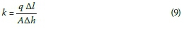
Prior to the opening of the outlet valve, full hydrostatic pressure corresponding to the depth of the seepage column will occur throughout the column. The distribution of hydrostatic pore pressure and potential (total head) is illustrated in Figure 1. During a hydraulic conductivity test, opening of the outlet valve results in the pore pressure at the bottom of the seepage column dropping rapidly to the head maintained at the outlet (in the case of Figure 1 it is atmospheric). The base of the column is usually taken as the test datum, so that the hydrostatic potential at the outlet is maintained at zero during flow and the pressure head and potential distributions change, as shown in Figure 1. In the case of a falling head test, the drop in potential, reflected by the drop in water level over a period of time (Δt), is subsequently recorded and the hydraulic conductivity is calculated using Equation 8.

 

 

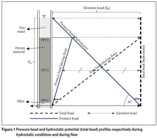
In Equation 8 L is the height of the specimen of porous material in the column, h₀ the original hydrostatic potential measured from the datum level and h₁the potential after time Δt. Equation 8 assumes a seepage column of constant cross-sectional area. Examining Equation 8 in the context of a hydraulic conductivity test carried out in a centripetal acceleration field leads to a number of observations:

■ In the derivation of the expression the initial hydraulic gradient was taken as h₀/L reducing over time (Δt) to h₁/L under free drainage. For the expression to be valid there may not be any obstruction to the flow, e.g. an outlet that is too narrow. Should such constrictions occur, the measured hydraulic conductivity will reflect this influence and the measurement will not be a result of only the material's hydraulic conductivity.

■ The centripetal acceleration exerted by the centrifuge is not reflected in this expression, as it cancels out when calculating the ratio h₀/h₁. The expression will therefore not be able to capture the increased potential energy per unit volume of water provided by the increase in acceleration. However, the time for a given drop in potential (Δh) will reduce as acceleration is increased. This will have the consequence that the hydraulic conductivity calculated using this expression will appear to increase linearly with increasing acceleration, as reported by Singh and Gupta (2000), i.e. k_m= N k_p.

■ The height of a seepage column can be significant, relative to the radius of the centrifuge. Centripetal acceleration is a function of the radial distance from the axis of rotation. In columns which are tall, relative to the radius of the centrifuge, the variation in acceleration with depth along the height of the column will be significant and should be considered.

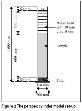
In a constant head hydraulic conductivity test, the hydrostatic potential at the upstream end of the sample is maintained at a constant level, the outlet control valve is opened and the resulting flow rate (q) monitored. In addition, the drop in hydrostatic potential (Δh) between known points, separated a known distance (Δl) along the length of the sample, has to be measured to enable the hydraulic conductivity to be calculated directly from Darcy's equation, Equation 9.

The hydrostatic potential can be monitored using standpipes, but they are difficult to record in the centrifuge. Alternatively, electronic pore pressure transducers can be used, usually more convenient in a centrifuge model.

In Equation 9 A is the cross-sectional area of the seepage column.

The following observations regarding hydraulic conductivity calculations using Equation 9 can be made:

■ It is not necessary to have free drainage through the material in the seepage column. Should a constriction occur, the effect will be reflected in the pore pressure measurements, and the correct hydraulic conductivity will still be calculated.

■ Should the hydrostatic potential difference (Ah) be measured as the physical difference in standpipe water levels, Equation 9 will produce results similar to that of Equation 8, i.e. the hydraulic conductivity will be found to increase with increasing acceleration, or k_m= N k_p. However, should the hydrostatic potential be calculated from the actual pressures recorded by pore pressure transducers, the hydraulic conductivity found will be that measured at normal gravity, assuming that compaction of the soil under increased acceleration is insignificant.

■As in the case of a falling head test, the height of the seepage column relative to the centrifuge radius has to be considered. A number of seepage column tests on two different materials are presented below, and the implications of the method in which the results are analysed are evaluated.

 

SEEPAGE COLUMN EXPERIMENTS

Centrifuge seepage column

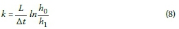
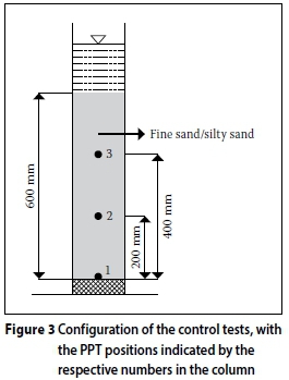
Considering the space available on the centrifuge platform, a 144 mm internal diameter perspex cylinder of 1 000 mm in height was selected as the model container. The model set-up, illustrated in Figure 2, included a 50 mm thick filter at the base, up to a 600 mm tall soil sample on top of the filter and a 300 mm head of water above the sample. To drain the cylinder, two remotely controlled valves were provided at the base. Two valves were provided as it was assumed that a single outlet would unacceptably restrict the outflow.

 

 

Pore pressure transducers

Small electronic pore pressure transducers (PPTs) were used to monitor the pore water pressures at discrete points within the sample during flow. From the pore pressure values the hydraulic gradient, and hence the conductivity of the material between the PPTs could be calculated.

Test configurations and procedures

Using the centrifuge model, flow through two homogeneous soil samples was assessed using falling head hydraulic conductivity tests conducted at two acceleration levels. Prior to testing, material was deposited to 600 mm above the filter. Three PPTs, spaced at 200 mm intervals, were placed in the sample (see Figure 3). The granular material had to be saturated to prevent the PPTs from desaturating before testing. This was accomplished by first filling the cylinder with de-aired water up to the level where the PPT would be placed. The dry granular material was then poured into the de-aired water and allowed to settle around the PPTs. The placement method resulted in low sample densities. It was the intention to study changes in hydraulic conductivity resulting from compaction during centrifugal acceleration.

 

 

After preparation, the model was placed on the centrifuge platform, the PPTs connected to the data acquisition system and the solenoid valves coupled to the power supply system. A small web camera was positioned to monitor the fall in water level within the seepage column to allow results to be recorded manually against time.

Material properties

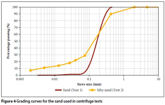
The grading curves for the two materials tested are presented in Figure 4. For Test 1, the material used was a poorly graded fine sand with a D₅₀ size of 0.17 mm. The material for Test 2 was a silty sand with a D₅₀ size of 0.14 mm and had a greater fraction of fine (silt and clay) material.

 

 

Tests conducted

Test 1 was carried out at an acceleration of 23 g and repeated at normal gravity (1 g). Once at 23 g, excess pore pressures were allowed to dissipate (stabilise) as the sample consolidated. The initial water level (h₀) was recorded and the solenoid valves opened to initiate the falling head test. After the water level had dropped somewhat, the outlet valve was closed and hydrostatic conditions allowed to re-establish, followed by a second flow stage. After the second stage, the solenoid valves were closed and the pore pressures were allowed to stabilise before the centrifuge was stopped. Once the centrifuge had stopped, the sample thickness and final water level were recorded.

The cylinder was subsequently filled with de-aired water, and a falling head test was conducted at 1 g, allowing the water level to drop by the same amount as in the centrifuge test.

For Test 2 similar procedures were followed as for Test 1, but acceleration was conducted to 29 g. (A different acceleration was applied in this test to model prototype layers of different thickness - details fall outside the scope of this paper). The flow rate was significantly slower due to the greater fraction of finer material in the sample. Consequently, only a single falling head test was conducted in the centrifuge and no 1 g test was conducted, as it became impractical due to the low hydraulic conductivity of the material.

 

ANALYSIS OF RESULTS

Calculating representative centripetal acceleration

The inertial acceleration (a) applied by the centrifuge is a function of the radius (r) of a point measured from the axis of rotation and the angular velocity (ω) of the centrifuge (Equation 10).

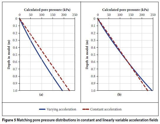
In a situation where the inertial acceleration is constant, the pore pressure (P) will vary linearly with depth (h) in the model according to Equation (11) (see Figure 5(a)).

 

 

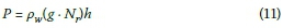
In Equation 11 N_ris the required centripetal acceleration which depends on the scale of the model, ρ_wis the density of water, g is gravitational acceleration and h indicates the depth in the model.

In the centrifuge, the inertial acceleration varies non-linearly along the height of a centrifuge model. Consequently, the pore pressures will vary non-linearly with depth throughout the model. Equation 12 accounts for the varying acceleration with depth in the model and is used to calculate the pore pressure at any given point (r).

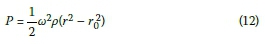
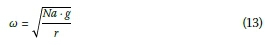
In Equation 12 r₀ is the radial distance from the axis of rotation to the model's free water surface and ω is calculated according to Equation 13. N_ais the set centripetal acceleration in multiples of gravitational acceleration.

The pore pressure distribution plotted using Equation 12 in Figure 5(a) illustrates that the water pressure distributions for a varying and constant inertial acceleration do not align. The centripetal acceleration is usually adjusted to ensure that the amount of under-stress relative to the linear stress distribution is equal to the amount of over-stress. This is achieved when the radial distance in Equation 13 is set to r₀ + H/3, with H the depth of soil in the model (Schofield 1980). Stresses will then match at a depth of 2/3H below the model surface, and N_awill represent the corresponding model scale. As demonstrated by Figure 5(b), the stress distributions do not match perfectly and there is both some over and under-stress. However, the deviations are relatively small and are normally considered insignificant.

Processing pore pressure data for hydraulic conductivity determination

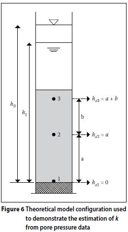
A practical example, using a hypothetical model configuration illustrated by Figure 6, is included to demonstrate the calculation of hydraulic conductivity values from the pore pressure measurements. In Figure 6 three PPTs are separated by distances a and b, and the initial and final heads recorded before and after a test are denoted by h₀ and h₁ respectively.

 

 

Following Bernoulli's equation (Equation 1), the total head (H) at any point is the sum of the pressure head (h_p) and the elevation head (h_z) when flow velocity is disregarded. Under hydrostatic conditions, before flow is initiated, the total head (or hydrostatic potential) at any point in the cylinder is equal to the total head at the bottom of the cylinder where the maximum pore pressure is measured. Therefore:

H₁= H₂= H₃.

As the acceleration varies with radial distance from the centrifuge axis, the elevation head cannot be simply taken as its elevation above the datum. Using the measured hydrostatic pore pressures for each PPT (h_p) and the total head (H₁), the elevation head (h_z) for each PPT can be calculated from Equation 14, as illustrated, for example, for PPT 2.

Provided that the material does not compress significantly during testing, these elevation heads remain constant for the duration of a test and are required for the determination of the hydrostatic potential, together with the pore pressure changes during flow, as illustrated for PPT 2 in Equation 15.

Therefore, the hydrostatic potential at each PPT during flow can be determined, and the difference in potential (AH) between two individual PPTs calculated, to determine the hydraulic conductivity between two PPTs from Darcy's law (Equation 16).

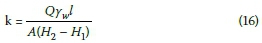
where l is the distance separating two PPTs. The average volumetric discharge rate (Q) is determined using the internal area (A) of the cylinder and the recorded fall in head over the duration of the test (h₀to h₁), provided that the fall in head is small. In Equation 16, H₂and H₁are expressed in units of pressure (e.g. kPa).

 

RESULTS

Pore pressure records from the centrifuge tests and calculated hydraulic conductivity values are presented and discussed below.

Test 1

The pore pressure records for the 23 g and 1 g tests are illustrated in Figure 7. After acceleration commenced, the pore pressures increased and stabilised rapidly once the required acceleration was reached, as shown in Figure 7(a). The pore pressure rapidly decreased once the solenoid valves were opened and flow commenced, as shown in Figure 7(b). Following the rapid pressure drop after opening the valves, the pore pressure decreased at a constant rate as the water level dropped. After closing the solenoid valves, hydrostatic conditions rapidly re-established at a lower head following the drop in the water level.

 

 

 

 

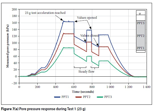
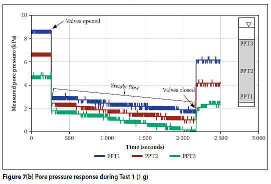
Despite differences in magnitude and timing, the trends in the recorded pore pressures for the 1 g test - Figure 7(b) - are similar to that of the 23 g test. Pore pressures and seepage velocities were much lower due to the test being conducted at 1 g. The jagged appearance of the graph is attributed to the PPTs measuring near the limit of their resolution.

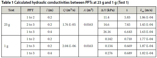
The water head decreased by a combined 0.237 m in 219 seconds over the two separate runs of the 23 g test. Flow was significantly slower for the 1 g tests and the water head fell by 0.240 m over 1 913 seconds. Potential differences (ΔH) between the PPTs were calculated from the pore pressures in Figures 7(a) and 7(b).

The volumetric discharge rate (Q) in each test was calculated from the drop in water level and the cylinder dimensions assuming constant flow. Hydraulic conductivity values between the PPTs were calculated using Darcy's equation (Equation 16) and are presented in Table 1. The values fell within the same order of magnitude with the hydraulic conductivity of the 1 g test, on average only 1.12 times greater than those of the 23 g test. Hence, the acceleration of the centrifuge appears to have had a minimal effect on the hydraulic conductivity, indicating that the material underwent only limited compression at high accelerations.

 

 

Test 2

The finer material in Test 2 was subjected to a greater acceleration of 29 g. The pore pressure response for Test 2 is illustrated in Figure 8. Initially the pore pressures increased as the centrifuge accelerated, and reached their maximum values at the test acceleration of 29 g. The pore pressures then gradually decreased, and stabilised as the material consolidated. Consolidation was first completed at PPT 3, followed subsequently by PPTs 2 and 1, reflecting their respective drainage path lengths.

 

 

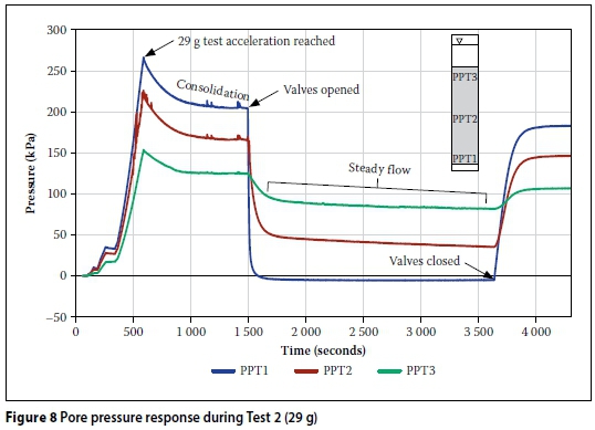
Once the pore pressures had stabilised, the valves were opened. As illustrated by Figure 8, PPT 1 showed the quickest response and the greatest drop in pore pressure, while PPT 3 measured the smallest pore pressure drop and took the longest to reach equilibrium after opening the valves. After the pressure drop following opening of the valves, the pore pressures decreased at a constant rate while steady flow occurred.

Despite the higher acceleration (29 g), the test took significantly longer than Test 1 (23 g). The water level reduced by 90.5 mm in 2 124 seconds. Consequently no 1 g test was conducted, as the rate of evaporation from the model was judged to be significant, relative to the low seepage rate.

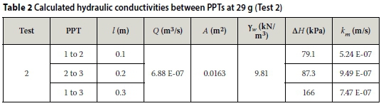
Hydraulic conductivity values, presented in Table 2, were calculated from the pore pressure data using Darcy's equation (Equation 16) as before. The values calculated for the sample do not vary significantly and all fall within the same order of magnitude.

 

 

DISCUSSION

Validity of Darcy's law in centrifuge tests

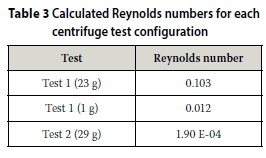
The hydraulic conductivities presented above assumes laminar flow, a requirement for Darcy's law to be valid (e.g. Fetter 2001; Singh & Gupta 2000). This requires the Reynolds number to be less than unity. Using a characteristic length corresponding to a D₁₀ of 0.85 mm for the sand (Test 1) and 0.004 mm for the silty sand (Test 2), Reynolds numbers (see Table 3) were calculated assuming the standard density and dynamic viscosity of water at 25°C and the specific discharge for each test. The Reynolds numbers fell well below unity, confirming the validity of Darcy's law.

 

 

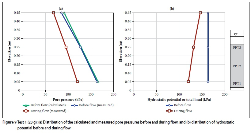
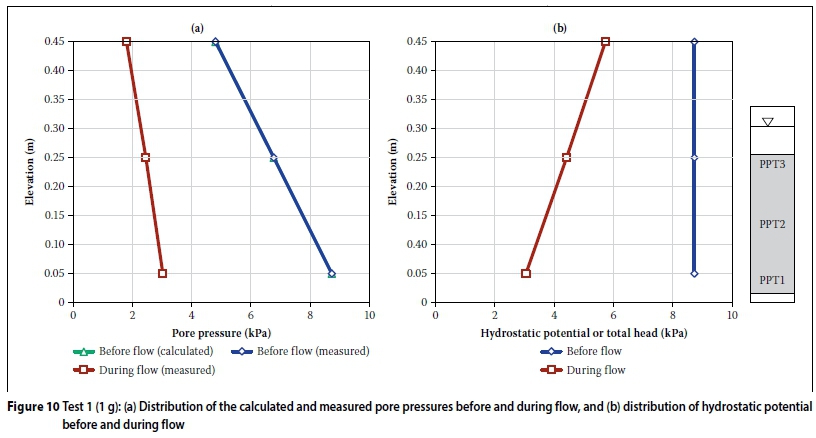
Centrifuge Test 1

The pore pressure and total head distributions for Test 1 at 23 g and 1 g are illustrated in Figures 9 and 10 respectively. The elevation of the seepage column outlet coincided with the bottom of the column. Under unobstructed flow the pore pressure at the bottom of the column should therefore have reduced to atmospheric when the outlet valves were opened. It can be seen from Figures 7, 9 and 10 that, after opening of the valves, the pressure head at the base of the column was still substantial, indicating that the outlet posed an obstruction to free flow. The falling head formulation for calculation of hydraulic conductivity is therefore not valid. Had the falling head formulation been used, a hydraulic conductivity of 2.2 E-05 m/s would have been calculated compared to the correct value of 1.6 E-04 m/s, a difference of an order of magnitude. Without pore pressure measurement at the base of the column, the user would not have been aware of this discrepancy.

The potential gradients at 23 g between respectively PPT 1 and PPT2, and PPT2 and PPT3, were very similar, indicating that the hydraulic conductivity of the material was not affected appreciably by compression under high acceleration.

A comparison of the results from the 1 g and 23 g tests in sand provided the opportunity to address the scaling law for hydraulic conductivity in the centrifuge. The flow rate in the 23 g test was significantly faster than in the 1 g test. Despite this difference, the calculated hydraulic conductivities from the 23 g test were on average only 1.12 times less than those at 1 g. This demonstrates that the hydraulic conductivity calculated from Darcy's law is not N times greater at an increased acceleration of N g. Clearly the pore pressures are increased N times at N g. The induced prototype pore pressures need to be dissipated over a flow path length that has been condensed N times in the centrifuge model. This supports the approach that the hydraulic gradient is scaled N times in the centrifuge, and not the hydraulic conductivity. This approach was also preferred by Taylor (1995), and Thusyanthan and Madabhushi (2003).

Centrifuge Test 2

Compared to Test 1, the pore pressures in Test 2 dissipated more slowly after the test acceleration had been reached, and the sample took considerably more time to consolidate (see Figure 8). Also, when the valves were opened, the pore pressures above the column base were notably slower to react than at the base, due to the lower hydraulic conductivity for the material in Test 2.

The pore pressure and total head distributions measured and calculated for Test 2 are presented in Figure 11. The elevation of the seepage column outlet was marginally below that of the bottom of the column. Once the outlet valves were opened, the pore pressure at the base of the column dropped to near atmospheric pressure, indicating that the outlet valve did not pose a restriction to flow. A true falling head test was therefore carried out, and both the falling head formula and Darcy's equation could therefore be used to assess the hydraulic conductivity. The hydraulic conductivities calculated using both approaches are summarised in Table 4, showing little difference.

 

 

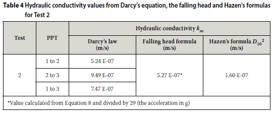
Figure 11(b) shows the hydrostatic potential gradient between PPT 1 and PPT 2 to be greater than between PPT 2 and PPT 3, indicating a lower hydraulic conductivity. This suggests that compression of the material under high accelerations resulted in a reduction in hydraulic conductivity.

The hydraulic conductivity values in Test 2 were two orders of magnitude lower than in Test 1. This was to be expected, given the respective grading curves (Figure 4). Hazen's formula predicted a similar value (see Table 4.)

 

CONCLUSIONS

The geotechnical centrifuge can be used to reduce the time necessary to conduct hydraulic conductivity tests on fine-grained granular materials. The increased acceleration imposed using the centrifuge serves to increase the potential energy per unit volume of water and therefore the hydrostatic potential driving flow. This results in an accelerated inter-particle flow velocity v_m = Nv_p where N is a multiple of gravitational acceleration. The time required to complete the test will also be accelerated by a factor N, assuming that the same volume of water flows through the sample.

In calculating hydraulic conductivity from the results of centrifuge tests, equations in which the increased hydrostatic potential does not feature (e.g. the falling head formula, Equation 8) will produce a hydraulic conductivity that appears to vary with the imposed acceleration level k_m= N k_p. On the other hand, should the actual hydrostatic potential as measured by, for example, pressure transducers, be incorporated into Darcy's equation (Equations 9 or 16), the calculated hydraulic conductivity should be the same as that calculated at normal gravity, provided that the material does not compress significantly under the increased acceleration in the centrifuge.

It is advocated that, in contrast with the recommendation by Singh and Gupta (2000) that hydraulic conductivity from a centrifuge test scales with the imposed acceleration, it can be assumed instead that it is the hydrostatic potential driving the flow which is increased by acceleration, leaving the calculated hydraulic conductivity unchanged compared to that measured under normal gravity.

When applying falling head formulas in which the actual hydrostatic potential is not explicitly incorporated, it is important to ensure that no obstruction to flow or other deviations from the assumptions made in the derivation of the equations are present, e.g. outlet valves restricting flow. Such obstructions will render the calculated hydraulic conductivities inaccurate. Without pore pressure measurement at the base of the column the user will not be aware of such obstructions. Equations catering for the actual hydrostatic potential, taking into account the acceleration level, and which are based on the actual flow rate, do not suffer from this shortcoming and can accommodate obstructed flow.

 

REFERENCES

Alyamani, M S & Sen, Z 1993. Determination of hydraulic conductivity from complete grain-size distribution curves. Ground Water, 31(4): 551-555.         [ Links ]

Bear, J 1972. Dynamics of Fluid in Porous Media. New York: Elsevier.         [ Links ]

Chakraborty, D, Chakraborty, A, Santra, P, Tomar, R K, Garg, R N et al 2006. Prediction of hydraulic conductivity of soils from particle-size distribution. Current Science, 90(11): 1527-1531.         [ Links ]

Culligan-Hensley, P J & Savvidou, C 1995. Environmental geomechanics and transport processes. In: Taylor, R N (Ed.), Geotechnical Centrifuge Technology, Glasgow: Blackie Academic and Professional, 196-264.         [ Links ]

Dell'Avanzi, E & Zornberg, Z G 2002. Scale factors for centrifuge modelling of unsaturated flow, In: Jucá, J F T, de Campos, J M P & Marinho, F A M (Eds.), Unsaturated Soils, Vol. 1. Lisse, Netherlands: A A Balkema, 425-430.         [ Links ]

Fetter, C W 2001. Applied Hydrogeology, 4th ed. Chapter 4: Principles of groundwater flow. Upper Saddle River, NJ: Prentice-Hall, 113-124.         [ Links ]

Hazen, A 1892. Some physical properties of sands and gravels. Massachusetts State Board of Health, Annual Report, 539-556.         [ Links ]

Kozeny, J 1927. Uber kapillare leitung des wassers im boden. Sitzungsberichte, Akademie der Wissenschaften in Wien, 136: 271-306.         [ Links ]

Nakajima, H & Stadler, A T 2006. Centrifuge modelling of one-step outflow tests for unsaturated parameter estimations. Hydrogeology and Earth System Sciences, 10: 715-729.         [ Links ]

Schofield, A N 1980. Cambridge Geotechnical Centrifuge Operations. Geotechnique, 30(3): 227-268.         [ Links ]

Singh, N & Gupta, A K 2000. Modelling hydraulic conductivity in a small centrifuge. Canadian Geotechnical Journal, 37(5): 1150-1154.         [ Links ]

Singh, N & Gupta, A K 2002. Modelling hydraulic conductivity in a small centrifuge: Reply 1. Canadian Geotechnical Journal, 39(2): 488-489.         [ Links ]

Taylor, R N 1995. Centrifuges in modelling: Principles and scale effects. In: Taylor, R N (Ed.), Geotechnical Centrifuge Technology, Glasgow: Blackie Academic and Professional, 19-34.         [ Links ]

Thusyanthan, N I & Madabhushi, S P G 2003. Scaling of seepage flow velocity in centrifuge models. Report No. CUED/D-SOILS/TR326, Cambridge University, Engineering Department.         [ Links ]

 

 

Correspondence:
W D van Tonder
Geology Department Hydrogeologist in Training
University of Pretoria Exxaro Resources Ltd
Pretoria 0001 PO Box 3583
South Africa Middelburg 1050
South Africa
T: +27 14 763 9945
E: warren.vantonder@exxaro.com OR warrenvt@hotmail.com

S W Jacobsz
Department of Civil Engineering
University of Pretoria
Pretoria 0001
South Africa
T: +27 12 420 3124
E: sw.jacobsz@up.ac.za

 

 

 

WARREN VAN TONDER, who graduated with an MSc in Hydrogeology from the University of Pretoria in 2016, is currently employed as a professional in training by Exxaro Resources. His work experience includes both underground and surface coal mining operations, and he is currently based at Grootegeluk Coal Mine in Lephalale (previously Elliras). His postgraduate studies focused on the physical modelling of fracture flow, as well as the permeability of coal mine backfill material, in the geotechnical centrifuge.

 

 

PROF SWJACOBSZ Pr Eng, MSAICE, graduated with an MEng degree in Civil Engineering from the University of Pretoria in 1996 and a PhD from the University of Cambridge in 2002. He is Associate Professor in the Department of Civil Engineering at the University of Pretoria. His research interests include physical modelling of geotechnical and soil-structure interaction problems in the geotechnical centrifuge.