


Servicios Personalizados
Articulo
 Inglés (pdf)
 Articulo en XML
 Referencias del artículo
Indicadores

Links relacionados
-
 Citado por Google
 -
 Similares en Google
Compartir

 Permalink
Journal of the South African Institution of Civil Engineering
versión On-line ISSN 2309-8775
versión impresa ISSN 1021-2019
J. S. Afr. Inst. Civ. Eng. vol.57 no.4 Midrand oct./dic. 2015
http://dx.doi.org/10.17159/2309-8775/2015/v57n4a1
TECHNICAL PAPER
Delay and queue lengths at stop/go control during half-width construction
L Venter; C J Bester
ABSTRACT
It is common practice in South Africa that road reseal projects, road reconstruction projects or road upgrade projects on two-lane, two-way roads are constructed in half-widths, resulting in a situation where traffic on the remaining roadway is reduced to one-way operation.
There is currently no method for determining a suitable length of work zone for half-width construction based on traffic volumes, and also no method for determining waiting time for the vehicle in the front of the stationary queue at the STOP/GO control, and of the back-of-queue position at such a work zone.
An Excel-based calculation sheet for determining the back-of-queue position and the maximum waiting time, was developed. This was used to develop design tables, graphs and equations that can be used by designers and contractors to estimate the back-of-queue position and maximum waiting time.
Based on the conclusions of this paper and the fact that this project was largely based on literature studies of traffic conditions not related to work zones for half-width construction, the main recommendation of the study is that all the input parameters which were investigated need to be verified and calibrated specifically for work zones for half-width construction.
INTRODUCTION
The definition of a "work zone for half-width construction" (work zone), in the context of this paper, shall be a "roadwork site for a rural two-way, two-lane road that is partially closed to traffic, where the remaining roadway is reduced to less than two lanes in width, for whatever reason, and where traffic is controlled manually at either end of such roadwork site by means of a STOP/ GO operation or temporary traffic signals to allow one-way traffic only, alternately in each direction, on the remaining roadway that is open to traffic". The impacts of the work zone for half-width construction on traffic operations will, however, extend beyond the work zone itself, i.e. into the approaches of the work zone for half-width construction.
Background
Waiting in a stationary queue at a work zone for half-width construction could be a frustration to motorists. In addition, motorists at the back of the queue cannot see the "maximum waiting time" displayed on the information traffic sign at the STOP/GO position and have no idea of how long they would have to wait.
During the design phase of a roads project, the engineer should devise a traffic management plan or traffic accommodation plan that would, inter alia, optimise site efficiency, traffic flow and all aspects of safety. Although it is not possible to predetermine how all construction sites will be managed during construction, because there are too many variables, it is considered very important that the engineer will plan, and work, in a systematic manner and in standardised steps to achieve the goals of the traffic accommodation plan, namely to optimise site efficiency, traffic flow and all aspects of safety. At a more detailed level, during the design phase, the engineer should identify the components of the construction site that would influence the traffic accommodation plan.
It is common practice in South Africa that road reseal projects, road reconstruction projects or road upgrade projects are constructed in half-widths. Whether the traffic, for a construction project, can be controlled by means of a STOP/GO operation or temporary traffic signals will depend largely on the environment, volume and speed of traffic, and on the length of the section of roadway subject to one-way control.
The length of the work zone for half-width construction is dependent on the time that a motorist would have to wait in the front of a stationary queue at a work zone for half-width construction, which in turn, is largely dependent on the volume and composition of traffic and the speed at which the vehicles can travel through the said work zone. It is therefore clear that the length of the work zone for half-width construction will differ from project to project, since the topography of the land through which the road traverses, and the volume and composition of traffic will determine the speed at which vehicles can travel through that work zone.
The COLTO Standard Specifications for Road and Bridge Works for State Road Authorities (COLTO 1998, pp 1500-5) Section 1513 (Accommodation of traffic where the road is constructed in half-widths), prescribe that:
a. The maximum length of half-width construction must be prescribed in the project specifications or on the drawings.
b. The maximum length of half-width construction shall not exceed 4 km, unless otherwise specified.
c. The minimum space between half-width construction sections shall be at least 2 km.
There is currently no method for determining a suitable length of work zone for half-width construction based on traffic volumes, and also no method for determining waiting time for the vehicle in the front of the stationary queue at the STOP/GO control, and of the back-of-queue position at such a work zone. In practice, practitioners easily use these prescribed values of 4 km and 2 km as a standard, irrespective of the site-specific or project conditions.
A safety issue related to work zones is that the first warning sign, in a series of signs for traffic accommodation for most traffic accommodation typical drawings, is the temporary "Roadworks ahead" warning sign (TW336), with a temporary information sign (TIN 11.3) that shows the distance to the work zone, i.e. the distance to the stop line at the STOP/GO position. These distances are normally shown as 600 m and 1 km. The combination of the temporary "Roadworks ahead" warning sign (TW336) and the temporary information sign (TIN 11.3) does therefore not make provision for the distance to the back-of-queue position at a work zone.
Back-of-queue positions can easily be longer than 600 m, or even 1 km, which means that arriving motorists are not alerted to the danger of possible stationary vehicles at the back-of-queue position, which could lead to back-of-queue collisions.
Previous publications
Previous international publications were mostly concerned with delay (total queue delay or average delay per vehicle) prediction and queue length (in vehicles) under one-way traffic control, but not specifically waiting time for the vehicle in the front of the stationary queue and back-of-queue position (in metres).
Cassidy and Son (1994) describe the adaptation and application of queueing models, originally derived for intersections controlled by vehicle-actuated traffic signals, to estimate delay at two-lane highway work zones. The models estimate expected delay as a function of directional traffic demand rates, work zone physical length and observed traffic measures.
Washburn et al (2008) provided a calculation procedure for estimating the capacity, delays and queue lengths of two-lane, two-way work zones with flagging control. This calculation procedure utilises a combination of standard signalised intersection analysis equations, as well as some custom models developed from simulation data.
Alternative methodologies
The Highway Capacity Manual (HCM) (TRB 2000) procedure determines delay per vehicle (in seconds per vehicle) and uses theoretical queue lengths to determine average back-of-queue (in vehicles), i.e. it does not use vehicle length and inter-vehicle space to determine back-of-queue position.
SIDRA1 intersection analysis programme, which is based on the HCM, calculates delay (total queue delay or average delay per vehicle) and average back-of-queue (in vehicles or metres).
These methodologies require cycle lengths and effective green time as input parameters, and do not take into account that the cycle length could be dependent on, amongst others, the length of work zone, the speed through the work zone or the dissipation time of the queue on the opposite side of a work zone for half-width construction, i.e. it makes no provision for one-way traffic only, alternately in each direction.
Objectives
The objectives of this paper, to determine the waiting time for the vehicle in the front of the stationary queue and back-of-queue position (in metres) at the STOP/GO control for a work zone for half-width construction, are as follows:
The first objective of this paper was to determine and investigate the factors that influence the waiting time for the vehicle in the front of the stationary queue at the STOP/GO control for a work zone for half-width construction.
The second objective of this paper was to develop equations to calculate the waiting time for the vehicle in the front of the stationary queue and the back-of-queue position.
The third objective was to use the aforementioned equations to develop design tables and graphs that could be used by designers and contractors for estimating the maximum waiting time for the vehicle in the front of the stationary queue and back-of-queue position.
Methodology
The following methodology was followed to achieve the afore-mentioned objectives:
a. Determine the variables that influence the waiting time for the vehicle in the front of the stationary queue at the STOP/ GO control for a work zone for half-width construction and back-of-queue position.
b. Investigate the variables that influence the waiting time for the vehicle in the front of the stationary queue at the STOP/GO control for a work zone for half-width construction and back-of-queue position by means of a literature study.
c. Develop an Excel-based calculation sheet for determining the back-of-queue position and the maximum waiting time for the vehicle in the front of the stationary queue.
d. Develop design tables and graphs that could be used by designers and contractors for estimating the back-of-queue position and maximum waiting time for the vehicle in the front of the stationary queue, at a work zone for half-width construction.
DETERMINING THE FACTORS THAT INFLUENCE WAITING TIME AND BACK-OF-QUEUE POSITION
Determining the sequence of a typical cycle for vehicles through a half-width construction work zone will help to determine the factors that influence the waiting time for the vehicle in the front of the stationary queue at the STOP/GO control and the back-of-queue position.
Waiting time for the vehicle in the front of the stationary queue
Let us assume that a vehicle arrives from direction "d" (the direction of analysis) at the stop line of a STOP/GO control for half-width construction. The time that this vehicle will have to wait at the stop line will depend on the following factors:
a. The time (t1in minutes) that it takes for the last vehicle that passed the stop line (i.e. the vehicle that was just in front of the vehicle that had to stop), in direction "d", to drive through the work zone. This time is dependent on the length (L in kilometres) of the work zone and the average speed in kilometres per hour) of that vehicle through the work zone. It can be written as:
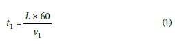
b. Once that vehicle has driven through the work zone and passes the point at the stop line at the far-side of the work zone, a few seconds may laps before the lane will be opened to the opposing traffic. This "operator lost time" (tL1in seconds) is attributed to the operator confirming that the last vehicle has passed the point at the stop line. The operator will then switch the traffic signal to green (or turn the STOP/GO sign) to indicate that it is safe for the vehicles to proceed.
c. "Start-up lost time" in seconds), which is the additional time consumed by the first few vehicles in the queue above and beyond the saturation headway, must also be considered. Start-up lost time accounts for the additional reaction time and vehicle acceleration time after the operator switched the traffic signal to green (or turned the STOP/GO sign).
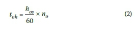
d. Following vehicles will then move past the stop line at a steady speed until the last vehicle in the original queue has passed the stop line. The saturation headway (hosin seconds) for these vehicles will be relatively constant and the total time (tohin minutes) that it takes for the queued vehicles to pass the stop line is equal to the saturation headway multiplied by the number of queued vehicles (no), in direction "o" (the opposing direction of analysis) that passed the stop line.
It can be written as:
e. "Added green time" (t ogin seconds) given by the operator to oncoming vehicles, in direction "o", joining the back of the original queue during the time that the moving queue is passing the stop line.
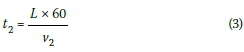
f. The time (t2in minutes) that it takes for the last vehicle that passed the stop line, in direction "o" (the opposing direction of analysis), to drive through the work zone. This time is dependent on the length of the work zone (L in kilometres) and the average speed (v2in kilometres per hour) of that vehicle through the work zone.
It can be written as:
g. Once that vehicle has driven through the work zone and passes the point at the stop line at the near-side of the work zone, a few seconds may laps before the lane will be opened to the opposing traffic. This "operator lost time" in seconds) is attributed to the operator confirming that the last vehicle has passed the point at the stop line and that it is safe to open the lane to the opposing traffic.
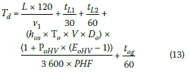
The total waiting time (Tdin minutes) for the vehicle, in direction "d" (the direction of analysis), in the front of the stationary queue, at the STOP/GO control for a work zone for half-width construction, can be written as:
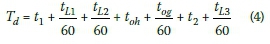
By substituting Equations 1 to 3 into Equation 4, the total waiting time (TJ) can be rewritten as:
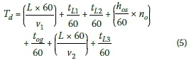
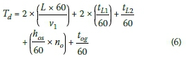
Assuming that the speeds of the last vehicles through the work zone, in both directions, are the same (v2= v2), and that the lost time, at both ends, for the operator to switch the traffic signal to green (or turn the STOP/GO sign), is the same (tL1= tL3 ) Equation 5 can be rewritten as:
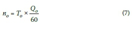
The number of queued vehicles (no) in direction "o" (the opposing direction of analysis) that arrived to form a queue at the far-side of the work zone is dependent on the uniform arrival rate (Qoin vehicles per hour) of vehicles in direction "o" during the time To(the total waiting time in minutes for the vehicle, in direction "o", in the front of the stationary queue at the STOP/GO control for a work zone for half-width construction) and can be written as:
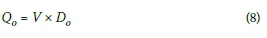
The uniform arrival rate (Qo in vehicles per hour) of vehicles in direction "o" is equal to the hourly two-way demand ( V in vehicles per hour) multiplied by the directional distribution, or directional split (Doexpressed as a decimal) of the hourly two-way volume on the road, and can be written as:
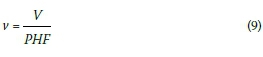
To convert the hourly two-way volume (V in vehicles per hour) to a design hourly two-way volume, it must be divided by the peak-hour factor (PHF the ratio of total hourly volume to the peak flow rate within the hour). The flow rate (v in vehicles per hour) based on a peak 15-minute period (i.e. the peak 15-minute flow multiplied by 4), which is also the design hourly two-way volume, can be written as:
The design hourly two-way volume should typically be chosen to incorporate seasonal or monthly fluctuations in traffic demand.
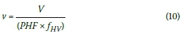
A conversion of the design hourly two-way volume in terms of passenger car equivalents (pce) can be computed using a heavy vehicle factor (fhv). The heavy vehicle factor accounts for the additional space occupied by heavy vehicles in the traffic stream and for the difference in operating capabilities of heavy vehicles compared to passenger cars. The design hourly two-way volume (v) can be written as:
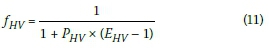
The heavy vehicle factor (fhv) adapted from the Highway Capacity Manual 2000 (HCM 2000) (TRB 2000, pp 22-7) is:
where:
Phv= proportion of heavy vehicles in the traffic stream, expressed as a decimal
EHV= the "passenger car equivalent for heavy vehicles - the number of passenger cars that is displaced by a single heavy vehicle of particular type under specified roadway, traffic and control conditions" (TRB 2000, pp 5-11).
By substituting Equations 7 and 8 into Equation 6, and by substituting the hourly two-way volume (v ) with the design hourly two-way volume of Equation 10 -, the total waiting time (Tdin minutes) can be rewritten as:
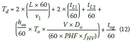
By including Equation 11, the heavy vehicle factor, in Equation 12, and expressing all the parameters in terms of the opposite direction "o", the total waiting time (Td) is rewritten as:
Similarly, it can be shown that the total waiting time (To) for the vehicle in direction "o", in the front of the stationary queue at the STOP/GO control for a work zone for half-width construction (assuming the start-up lost time tL2 is the same in both directions), can be rewritten as:
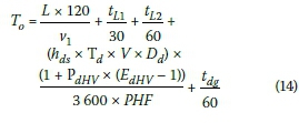
One important time parameter, namely added green time (togand tdg), in both directions "o" and "d", must be highlighted from Equation 13 and Equation 14.
During the time that it takes for the queued vehicles to pass the stop line, vehicles will arrive at the back of the queue to form part of the now "moving queue". The added green time is, in fact, the additional time needed for the additional vehicles, which were not part of the original stationary queue, to also pass the stop line.
It is therefore assumed that the operator will not "cut off" the moving queue after a certain number of vehicles have passed the stop line, but that all vehicles will clear the stop line before the operator will switch the traffic signal to red (or turn the STOP/GO sign), i.e. the end overflow queue will always be equal to zero. This assumption has a marked effect on the total waiting time (Td and To) in Equation 13 and Equation 14.
It is clear from Equation 13 that the total waiting time, Tj for the vehicle in the front of the stationary queue is dependent on the total waiting time, Toand vice versa for the total waiting time, Toin Equation 14.
When the added green time, tggin Equation 13 increases, the total waiting time, Tj will increase, hence the total waiting time, Toin Equation 14 will also increase. When the total waiting time, Toincreases, more vehicles will accumulate in the stationary queue, in direction "o", which means that more vehicles will have to pass the stop line; and more vehicles will arrive, during that time, at the back of the moving queue; and even more added green time, togwill be needed; and vice versa for the added green time tdg
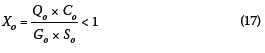
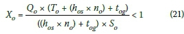
The total waiting time (Tdand To) in Equation 13 and Equation 14 will therefore have to be solved by means of an iterative process, whereby green time (togand tg is added, in both directions "o" and "d", until an equilibrium is reached. This equilibrium can only be reached under circumstances where the traffic demand (uniform arrival rate Q in veh/s) is less than the maximum flow rate (saturation flow or departure rate S in veh/s) that can pass the stop line, for each direction "o" and "d". The ratio of traffic demand to the maximum flow is defined as the degree of saturation (X), and is based on the principles of "fixed time traffic signals" as described by Van As and Joubert (2000, p 8.3.1), as follows:
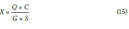
where:
Q = traffic demand or uniform arrival rate (veh/s)
C = total cycle length time (s)
G = effective green time (s)
S = saturation flow or departure rate (veh/s).
Under circumstances where the traffic demand is less than the saturation flow rate, i.e. the degree of saturation is less than one (X < 1), the approach at the stop line is "undersaturated".
Equation 15 can be rewritten for each direction "d" and "o" as:
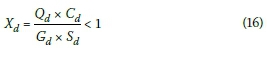
and
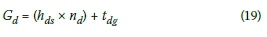
The total cycle length (C in seconds) for each approach is equal to the effective red time (R in seconds) plus the effective green time (G in seconds). The effective red time for each approach is equal to the total waiting time (Tj and To) in Equation 13 and Equation 14; and the effective green time for each approach is equal to the total time that it takes for the queued vehicles to pass the stop line (see Equation 2) plus the added green time. Therefore:
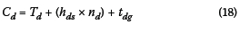
and
Equation 16 can be rewritten as:
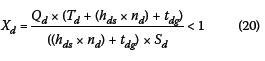
Similarly, Equation 17 can be rewritten as:
The traffic demand (Qj and Qoin veh/s) and the number of vehicles (nj and no) that passed the stop line in Equations 20 and 21 can be substituted with Equations 7 to 11, in both directions "d" and "o", for design volumes.
The iteration process, whereby green time (togand tdg) is added, in both directions "o" and "d" to solve the total waiting time (Tj and To) in Equation 13 and Equation 14, will have to be repeated and checked against the degree of saturation, until an equilibrium is reached where the degree of saturation in both directions is less than one.
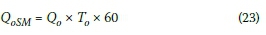
Back-of-queue position
The maximum stationary queue length (Qsmin veh) is equal to the traffic demand (uniform arrival rate, Q in veh/s) that arrives during the effective red time for each direction, where the effective red time for each approach is equal to the total waiting time (Tj and Toin min) in Equation 13 and Equation 14.
Therefore the maximum stationary queue length for each direction can be written as:
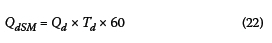
and
As vehicles in the front of the stationary queue start to move past the stop line, the vehicles at the back of the queue are still stationary, i.e. the back of the stationary queue is still at the same position, although there are now fewer cars in the actual stationary queue. At the same time, vehicles are arriving (at a uniform arrival rate, Q in veh/s) at the back of the stationary queue, i.e. the position of the back of the queue will keep growing until all the vehicles in the queue start to move.
"A shock wave is formed as vehicles disperse from the front of the stopped queue" (Van As & Joubert 2000, p 5.2.7). The speed at which the shock wave moves backwards from the front of the queue, as vehicles disperse from the front of the queue, can be calculated on the basis of the fundamental relationship between the three basic macroscopic characteristics that define traffic flow, namely speed, flow and density.
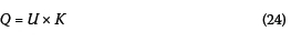
where:
Q = flow (veh/h)
U = macroscopic speed (km/h)
K = density (veh/km).
The speed of the shock wave can be written as:
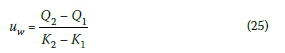
where:
uw= shock wave speed (km/h)
Q2= flow of dispersing vehicles (veh/h), which equals the saturation flow rate (S in veh/h)
Q1= flow of stationary vehicles (veh/h), which is equal to zero
K2= density of the dispersing vehicles (veh/km)
K1= density of stationary vehicles (veh/km).
Seeing that the density of stationary vehicles (veh/km) will always be more than the density of the dispersing vehicles (veh/km), the shock wave speed will be a negative value, i.e. the shock wave travels backwards.
The density of the dispersing vehicles (K2in veh/km) is equal to the saturation flow rate (S in veh/h) divided by the speed of the dispersing vehicles, which is taken as the average speed (vi km/h) of the last vehicle through the work zone.
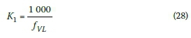
The density of stationary vehicles (Ki in veh/km) is equal to the inverse of the average vehicle length factor (fVLin m/veh) that takes the vehicle composition, the vehicle length (Liin metres) and the inter-vehicle space (siin metres) into account.
The average vehicle length factor ( fVLin m/veh) can be written as:
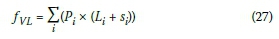
where:
Pi = proportion of type i vehicles in the traffic stream, expressed as a decimal
Li= the average length of type i vehicles in the stream (m)
si= average inter-vehicle spacing (m).
The density of stationary vehicles (Kiin veh/km) can be written as:
By substituting Equations 26, 27 and 28 into Equation 25, and dividing by the average vehicle length factor ( fVLin m/veh), the speed of the shock wave (uwsin veh/s) can be written as:
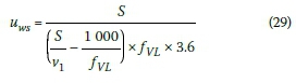
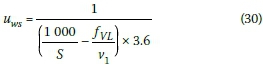
By further manipulation of Equation 29 and multiplying it by minus one (-1) to convert the speed of the shock wave to a positive value, the speed of the shock wave (uwsin veh/s) can be written as:
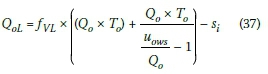
The maximum back-of-queue position (Qmin veh) is equal to the maximum stationary queue length (Qsmin veh), as shown in Equations 22 and 23, plus the traffic demand (uniform arrival rate Q in veh/s) that arrives during the additional time (dT in min) needed for the queue to disperse, i.e. the additional time for the shock wave to reach the back of the queue. This relationship can be written as:
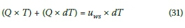
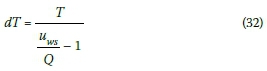
The additional time (dT in min) for the queue to disperse can be found by solving Equation 31:
The maximum back-of-queue position (QM in veh) for each direction can be written as:
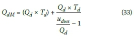
and
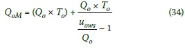
The maximum back-of-queue position (QL in metres) can be calculated by multiplying the maximum back-of-queue position (QMin veh) by the average vehicle length factor ( fVL in m/veh), from Equation 27, which takes the vehicle composition, the vehicle length (Li in metres) and the inter-vehicle space (siin metres) into account.
Since there would be one less inter-vehicle space than vehicles in the queue, one average inter-vehicle space must be subtracted from the equation when it is converted from maximum back-of-queue position (QM in veh) to maximum back-of-queue position (QLin metres).
The maximum back-of-queue position (QLin metres) can be written as:
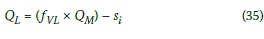
By substituting Equations 33 and 34 into Equation 35, the maximum back-of-queue position, in metres, for each direction can be written as:
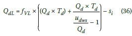
and
LITERATURE STUDY OF THE VARIABLES THAT INFLUENCE WAITING TIME AND BACK-OF-QUEUE POSITION
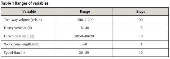
Two types of variables were identified in the preceding section. Firstly there are those that can be directly measured or derived from the specifications of the project, such as traffic volumes, composition and directional split, length of work zone, and speed of the last vehicle through the work zone. For the development of the design tables these will be the independent variables, and the ranges in which they will be used are shown in Table 1.
Secondly there are the variables that will be fixed for the development of the design tables. Their values are discussed below.
Operator lost time
The operator lost time (fL1and tL3) is attributed to the operator confirming that the last vehicle through the work zone has passed the point at the stop line and that it is safe to open the lane to the opposing traffic. A nominal 12 seconds for operator lost time was assumed, based on observations at various work zones for half-width construction sites in the Western Cape.
Start-up lost time
Start-up lost time (tL2) is the additional time consumed by the first few vehicles in the queue above and beyond the saturation headway. Bester and Varndell (2002) quoted from previous studies that start-up lost time ranged from 0.75 seconds to 3.04 seconds. It was assumed, for the calculation of waiting time and back-of-queue position, that start-up lost time at a work zone shall be a maximum of 3.0 seconds.
Saturation headway
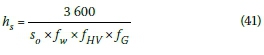
Saturation flow rate, according to the HCM 2000 (TRB 2000, pp 7-10), is defined as "the flow rate per lane at which vehicles can pass through a signalized intersection". When the saturation flow rate is determined from time measurements taken in the field, it is computed by Equation 38:
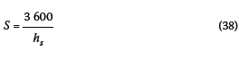
where:
S = saturation flow or departure rate(veh/h)
hs= saturation headway (s/veh).
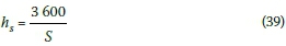
The saturation headway is described in the HCM 2000 (TRB 2000, pp 5-14) as "the average headway between vehicles occurring after the fourth vehicle in the queue and continuing until the last vehicle in the initial queue clears the intersection".
To determine saturation headway, Equation 38 can be rewritten as:
Since very little information on saturation flow rates for South African conditions could be obtained, which was affirmed by Bester and Meyers (2007), the saturation flow rate can be determined based on the estimation procedure described in the HCM 2000 (TRB 2000, pp 16-9 to 16-13) for signalised intersections, whereby a base saturation flow rate (so in pc/h), under ideal conditions, is used and adjusted for various factors that can influence traffic behaviour and in turn the saturation flow rate. Ideal conditions are described in the HCM 2000 (TRB 2000), but include some assumptions, namely 3.6 metre lane widths, no heavy vehicles in the traffic stream, flat gradient, etc.
The estimated saturation flow rate is calculated by adjusting Equation 16-4 of the HCM 2000 (TRB 2000, p 16-9) as follows:
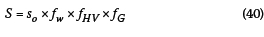
where:
S = saturation flow or departure rate (pc/h)
so= base saturation flow rate (pc/h)
fw= lane width factor
fHV= heavy vehicle factor
fG= gradient factor.
By substituting Equation 40 into Equation 39 the saturation headway (hsin s/veh) can be rewritten as:
Base saturation flow rate
The HCM 2000 (TRB 2000) suggests that a capacity of 1 600 pc/h/ln be used for short-term freeway work zones, irrespective of the lane closure configurations; and for long-term construction zones, capacity values range from 1 550 veh/h/ln (where traffic crosses over to lanes that are normally used by the opposing traffic), to 1 750 veh/h/ ln (where no crossover is needed, but only a merge down to a single lane - the value is typically higher).
Bester and Meyers (2007) derived an equation for saturation flow rate based on their study of saturation flow rates at different intersections under different circumstances in Stellenbosch in the Western Cape.
Their equation is as follows:
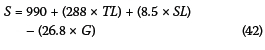
where:
S = saturation flow or departure rate (pc/h/ln)
TL = number of through lanes (1 or 2)
SL = speed limit (60 km/h or 80 km/h)
G = gradient (percentage), e.g. 3% would be 3.
By setting the number of through lanes to one, and the gradient to zero, Equation 42 can be rewritten as:
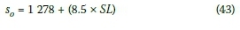
Equation 43 was used to determine base saturation flow rates (so in pc/h) at different speed limits, as shown in Table 2.
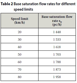
These base saturation flow rates in Table 2 need to be adjusted for various factors, as described above. It is assumed, for the calculation of waiting time and back-of-queue position, that the speed limit in Table 2 is equal to the average speed through the work zone.
Lane width factor
According to the HCM 2000 (TRB 2000, p 16-10) "the lane width adjustment factor fw accounts for the negative impact of narrow lanes on saturation flow rate and allows for an increased flow rate on wide lanes" and is given by:
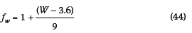
where:
W = lane width (m) for W > 2.4 m.
For the purpose of this paper a lane width of 3.1 m was used.
Heavy vehicle factor
Heavy vehicles reduce the saturation flow rate because of their lower acceleration rates and the fact that they occupy more road space, both in length and width (Van As & Joubert 2000), compared with passenger cars. The heavy vehicle factor (fhv) was given in Equation 11 as:
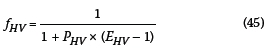
The calculation of the proportion of heavy vehicles (PHV) in the traffic stream should be based on vehicle classification sourced from project-specific or local data.
The passenger car equivalent for heavy vehicles (EhV) was chosen as 4.3 for the calculation of waiting time and back-of-queue position; and was kept constant for all calculations. This value is consistent with the average passenger car equivalent value quoted by Molina et al (1987, p 32), of 4.3 for a 5-axle heavy vehicle in the front of the queue at signalised intersections.
Gradient factor
"The gradient factor (fG) accounts for the effect of grades on the operation of all vehicles" (TRB 2000, p 16-10) at traffic signals, namely it is expected that negative gradients will increase saturation flow rates and positive grades will decrease saturation flow rates.
Bester and Meyers (2007) concluded that the departure gradients at intersections have a much greater effect on the saturation flow rate locally than in the USA. They derived an equation for the gradient factor (fG) based on their study of saturation flow rates at different intersections under different circumstances in Stellenbosch in the Western Cape, as follows:
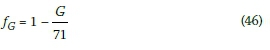
where:
G = departure gradient (percentage), e.g. 3% would be 3.
Added green time
"Added green time" (tg) is the additional time given by the operator to allow any additional oncoming vehicles, over and above the original stationary queued vehicles, to pass the stop line.
It is therefore assumed that the operator will not "cut off" the moving queue after a certain number of vehicles have passed the stop line, but that all vehicles will clear the stop line before the operator will switch the traffic signal to red (or turn the STOP/GO sign), i.e. the end overflow queue will always be equal to zero.
Average length of type of vehicles in the stream
The average length (L;) of type of vehicles in the traffic stream should be based on information sourced from project-specific or local data.
The SIDRA intersection analysis programme uses an average vehicle length of 5.1 m for light vehicles and 11.0 m for heavy vehicles in its "USA model", and an average vehicle length of 4.5 m for light vehicles and 10.0 m for heavy vehicles in its "Standard model" (e.g. as it applies to Australia).
The average vehicle length of 4.38 m and 12.55 m, for light and heavy vehicles respectively, were used to calculate the waiting time and back-of-queue position. These values for average vehicle lengths were based on the data of a seven-day electronic traffic count (approximately 48 400 vehicles for the seven days) on the R45 near Malmesbury, in the Western Cape, in 2010.
Average inter-vehicle spacing
The inter-vehicle spacing (s) is the distance or space, in metres, between vehicles (rear bumper of one vehicle to front bumper of the following vehicle).
Long (Long 2002, p 86) concluded that
"from observations measured at a variety of sites (in the USA), inter-vehicle spacings were found to average 3.66 m (12 ft) and were not found to differ significantly at different sites."
The average inter-vehicle spacing of 3.66 m between all vehicles was used to calculate the waiting time and back-of-queue position at a STOP/GO control for a work zone for half-width construction.
DEVELOPMENT OF DESIGN TABLES AND GRAPHS
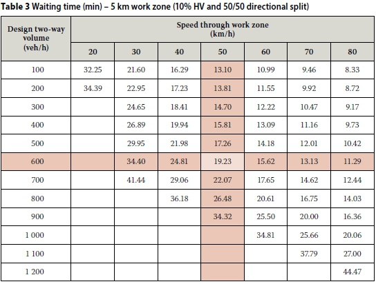
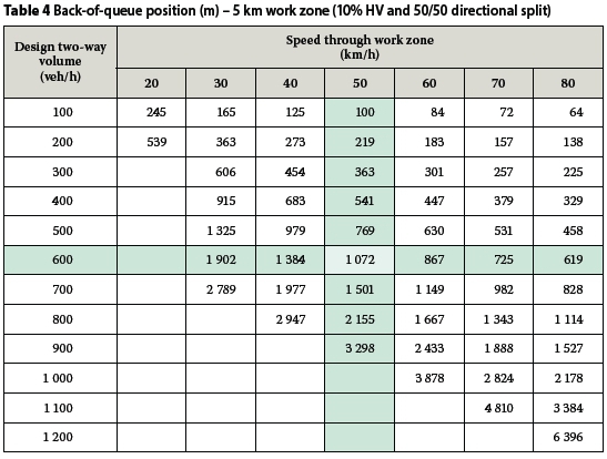
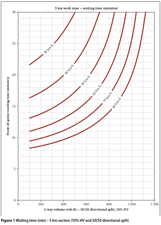
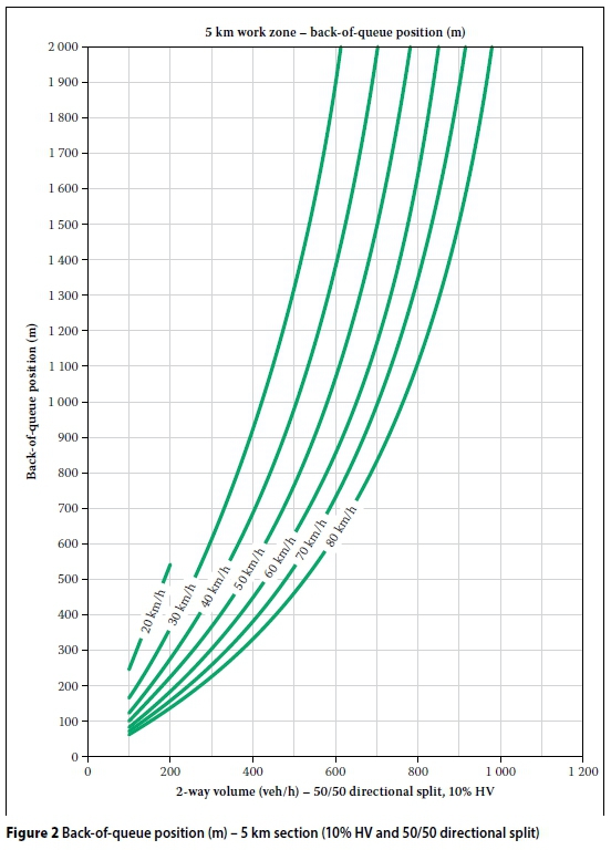
By using the iterative procedure in the Excel-based calculation sheet it was possible to develop design tables and graphs to show the waiting time at the front of the queue and the back-of-queue position for different design volumes, work zone lengths, speeds through the work zone, directional splits and percentages of heavy vehicles. All other input variables were fixed at the values given in the previous section. Examples of such tables and graphs are given in Tables 3 and 4, and Figures 1 and 2. From these it can be seen that for a two-way design volume of 600 veh/h, 10% HVs, a 50/50 directional split and a speed of 50 km/h (the 15th percentile heavy vehicle speed), a 5 km work zone will cause a 19.23 minutes waiting time and a back-of-queue position of 1 070 m from the stop line.
SENSITIVITY ANALYSIS OF INPUT VARIABLES FOR THE CALCULATION OF WAITING TIMES AND BACK-OF-QUEUE POSITIONS
The sensitivity analysis was built around a typical work zone scenario with 600 veh/h two-way design volume, 10% heavy vehicles, 60/40 directional split, 3 km work zone length and 50 km/h speed through the work zone. The sensitivity analysis did not make allowance for changes to average vehicle spacing (average vehicle length and inter-vehicle space), lane width, passenger car equivalent value, departure gradient, start-up lost time and operator lost time. The results are shown in Tables 5 to 9.
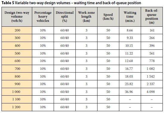
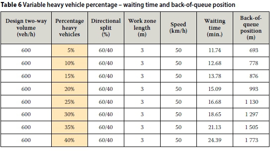
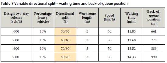
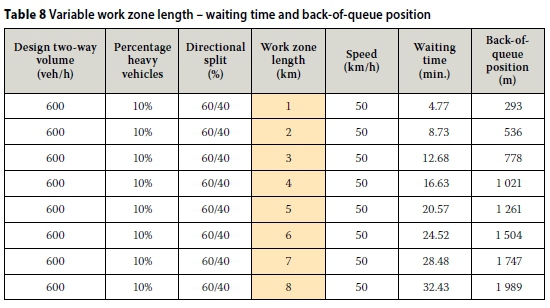
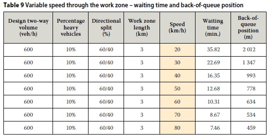
From the sensitivity analysis it was found
that:
■ Waiting time and back-of-queue position exponentially increase with an increase in the traffic volume and the percentage of heavy vehicles.
■ The effect of directional split is not significant.
■ Waiting time and back-of-queue position increase linearly with the length of work zone.
■ Waiting time and back-of-queue position decrease linearly with the speed through the work zone.
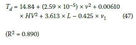
REGRESSION ANALYSIS
The data from Tables 5 to 9 were used in a regression analysis to derive equations for practitioners to approximate the total waiting time and back-of-queue position as follows:
The total waiting time (min):
And the back-of-queue position (m):
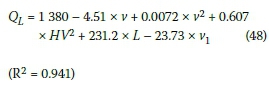
where:
v = design hourly two-way volume (veh/h)
HV = percentage heavy vehicles, e.g. 10% would be 10
L = length of work zone (km)
v1= average speed through work zone(km/h).
It should be noted that the above are only valid for the ranges used in the sensitivity analysis.
COMPARISON OF RESULTS
A brief comparison of the results from Tables 3 and 4 (for two-way design volume of 600 veh/h and 50 km/h) against a SIDRA analysis (where the cycle length and effective green times were converted from the Excel-based calculation sheet to the SIDRA input parameters) showed reasonably comparable values within a range of ± 15%. The SIDRA analysis results were found to be lower than the tabled values for two-way design values above 600 veh/h, and higher for two-way design values below 600 veh/h.
Although the SIDRA analysis results seemed reasonably comparable with the Excel-based calculation sheet, it should not be used as a validation of the equations or the parameters that were used in this paper, since the parameters in the Excel-based calculation sheet had to be converted to the input parameters used by SIDRA.
CONCLUSIONS AND RECOMMENDATIONS
This paper examined the factors that influence the waiting time for the vehicle in the front of the stationary queue at the STOP/ GO control, and back-of-queue position, at a work zone for half-width construction. An Excel-based calculation sheet for determining the back-of-queue position and the maximum waiting time for the vehicle in the front of the stationary queue was developed. This was used to develop "design tables" and "quick design graphs" that could be used by designers and contractors to estimate the back-of-queue position and the maximum waiting time for the vehicle in the front of the stationary queue.
Based on this paper, the following can be concluded:
■ Very little information is available or documented in South Africa to accurately determine the back-of-queue position and waiting time for the vehicle in the front of the stationary queue at the STOP/GO control for a work zone with half-width construction.
■ Waiting time and back-of-queue position exponentially increase with an increase in the traffic volume and the percentage of heavy vehicles.
■ The effect of directional split is not significant.
■ Waiting time and back-of-queue position increase linearly with the length of work zone.
■ Waiting time and back-of-queue position decrease linearly with the speed through the work zone.
■ The waiting time and back-of-queue position could be estimated by using the Excel-based calculation sheet. This can be used to determine the position of advance warning signs at a work zone.
■ The Excel-based calculation sheet could also be utilised to find the optimum work zone length, based on the project parameters, to comply with predetermined criteria for, for example, maximum waiting time of 20 min or maximum back-of-queue position of 2 km.
Based on the conclusions of this paper, and the fact that it is largely based on literature studies of traffic conditions not related to work zones for half-width construction, the most important recommendation is that all the input parameters which were used need to be verified and calibrated against field data pertaining specifically to work zones for half-width construction.
A second recommendation is that the "Temporary Congestion" warning sign "TW355", either as a VMS or not, should be used approximately 150 m in advance of the back-of-queue position at work zones.
The validation of the outcomes of this paper could be used in the economic analysis of roads projects. For example, economic cost of delays, based on daily volumes and typical daily volume distribution graphs, could be used to determine the cost-effectiveness of stop-go versus the construction cost of a bypass.
NOTE
1 SIDRA SOLUTIONS software products developed by Akcelik & Associates (Pty) Ltd.
REFERENCES
Bester, C J & Meyers, W L 2007. Saturation flow rates. Paper presented at the 26th Annual South African Transport Conference (SATC 2007), Stellenbosch: University of Stellenbosch, 9-12 July. [ Links ]
Bester, C J & Varndell, P J 2002. The effects of leading green phase on start-up lost time of opposing vehicles. Paper presented at the 21st Annual South African Transport Conference (SATC 2002), Stellenbosch: University of Stellenbosch, 15-19 July. [ Links ]
COLTO (Committee of Land Transport Officials) 1998. Standard Specifications for Road and Bridge Works for State Road Authorities. Midrand: SAICE. [ Links ]
Cassidy, M J & Son, Y T 1994. Predicting traffic impacts at two-lane highway work zones. West Lafayette, IN, US: Purdue University. [ Links ] Long, G 2002. Intervehicle spacings and queue characteristics. Transportation Research Record, 1796: 86-96. [ Links ]
Molina, C J, Messer, C J & Fambro, D B 1987. Passenger car equivalents for large trucks at signalised intersections. College Station, TX, US: Texas Transportation Institute. [ Links ]
TRB (Transportation Research Board) 2000. Highway Capacity Manual. Washington D.C.: Transportation Research Board of the National Academies. [ Links ]
Van As, S C & Joubert, H S 2000. Traffic flow theory. Draft 2000 edition used as class notes for the course- based Master's Degree programme in Transportation Engineering at Stellenbosch University. Pretoria: University of Pretoria. [ Links ]
Washburn, S S, Hiles, T & Heaslip, K 2008. Impact of lane closures on roadway capacity: Development of a two-lane work zone lane closure analysis procedure (Part A). Gainesville, FL, US: University of Florida. [ Links ]
 Correspondence:
LOUW VENTER
AECOM SA (Pty) Ltd
PO Box 112 Bellville
7535
South Africa
T: +27 (0)21 950 7500
E: Louw.Venter@aecom.com
CHRISTO BESTER
Department of Civil Engineering
Stellenbosch University
Private Bag X1
Matieland
7602
South Africa
T: +27 (0)21 808 4377
E: cjb4@sun.ac.za

LOUW VENTER Pr Eng is an Associate at AECOM SA (Pty) Ltd and has 15 years' experience in the field of Transportation Engineering. He obtained the degree BEng (Civil) from Stellenbosch University in 1999 and MEng cum laude, specialising in Transportation Engineering, also from Stellenbosch University in 2014. His key areas of experience include geometric design, transport planning and transport economics, contract administration and project management.
PROF CHRISTO BESTER Pr Eng is a Fellow of SAICE and emeritus professor in the Department of Civil Engineering at Stellenbosch University. He obtained a BSc, BEng and MEng at Stellenbosch University and a DEng at the University of Pretoria. He worked for consultants and the CSIR before joining Stellenbosch University in 1994. His research focuses on Traffic Engineering and Road Safety.

