TECHNICAL PAPER

 

Uncertainty evaluation with fuzzy schedule risk analysis model in activity networks of construction projects

 

 

Ö Ökmen; A Öztaş

Correspondence

 

 

---

ABSTRACT

Construction projects are prone to uncertainty due to various risk factors, such as unexpected weather conditions and soil properties. Depending on this, the actual duration of activities frequently deviates from the estimated duration time in either favourable or adverse directions. For this reason, evaluation of uncertainty is required to make the correct decisions when managing construction project network schedules. In this regard, this paper presents a new computer-aided schedule risk analysis model - the Fuzzy Schedule Risk Analysis Model - to evaluate uncertain construction activity networks when activity duration and risk factors are correlated. The proposed model utilises Monte Carlo Simulation and a fuzzified Critical Path Method procedure conducted by fuzzy sets and fuzzy operations. The paper also includes an example application of the model to a housing project. The findings of this application show that the model operates well and produces realistic results in capturing correlation indirectly between activity durations and risk factors regarding the extent of uncertainty inherent in the schedule.

Keywords: construction management, scheduling, fuzzy sets, simulation modelling, risk analysis

---

 

 

INTRODUCTION

It is possible to show the dependency relationships between activities, detect the critical activities, compute the float times, level the resources, and find the shortest project duration with the popular project network scheduling method, the Critical Path Method (CPM) (Griffis & Farr 2000; Halphin & Woodhead 1998; Oberlender 2000). However, CPM is a deterministic method, due to the crisp values used to represent the activity durations, and therefore it is not possible to evaluate the effect of uncertainty on construction schedules with CPM. Various risk factors affect construction projects and it is not possible to estimate the activity durations with certainty in advance. This causes CPM to misidentify the critical paths and project durations (Jaafari 1984). Construction activity networks are influenced by uncertainties related to risk factors such as weather conditions, design faults, scope changes, site conditions and soil properties (Edwards 1995; Flanagan & Norman 1993). Furthermore, all of the possible risk factors in a construction project might be schedule risks, because they are related to the schedule directly or indirectly. Due to the uncertainty effect, uncritical activities determined by CPM might be critical in practice.

In order to evaluate the uncertainty effect on construction activity networks, researchers have developed nondeterministic scheduling methods, such as the Program Evaluation and Review Technique (PERT) (Dept of the Navy 1958), the Probabilistic Network Evaluation Technique (PNET) (Ang et al 1975) and the Monte Carlo Simulation (MCS) (Diaz & Hadipriono 1993). These methods are capable of analysing uncertainty, but they are insufficient in identifying the sensitivity of activities individually or the network as a whole to risk factors. Furthermore, they ignore the correlation effect between activities (Wang & Demsetz 2000a,b). They approach the uncertainty problem through accepting the activity durations between some estimated boundary values and trying to measure the variance of project completion time. However, in cases where several activities are influenced by the same risk factor at different levels, their durations are correlated in compliance with these levels. If the activities on a path are correlated, the variability of the path's duration would increase, and depending on this, the project completion date would be highly uncertain, due to the uncertainty in path durations (Wang & Demsetz 2000b).

Fuzzy logic and fuzzy modelling have been utilised in many papers related to civil engineering applications (Chao 2007; Stathopoulos et al 2008; Jin & Doloi 2009; Sadeghi et al 2010). Furthermore, various schedule risk analysis models can be found in the literature, such as Model for Uncertainty Determination (MUD) (Carr 1979), Project Duration Forecast (PRODUF) (Ahuja & Nandakumar 1985), PLATFORM (Levitt & Kunz 1985), Conditional Expected Value Model (CEV) (Ranasinghe & Russell 1992), Exact Simulation (Touran & Wiser 1992), Factored Simulation (Woolery & Crandall 1983), Networks under Correlated Uncertainty (NETCOR) (Wang & Demsetz 2000b), Network Evaluation with Correlated Schedule Risk Analysis (CSRAM) (Ökmen & Öztaş 2008) and Judgmental Risk Analysis Process (JRAP) (Öztaş & Ökmen 2005). All of these methods are risk factor based and they capture the correlation, either directly by using correlation coefficients or indirectly by using qualitative data. While some of them consider both the favourable and the adverse effects of risk factors, some consider only the adverse effects. However, none considers the correlation between risk factors.

This paper presents a new computer-aided schedule risk analysis model - the Fuzzy Schedule Risk Analysis Model (FSRAM) - to evaluate construction activity networks under uncertainty when activity durations and risk factors are correlated. The paper also includes an example application of the model to a housing project.

FSRAM utilises MCS and a fuzzified CPM procedure conducted by fuzzy sets and fuzzy operations. Activity durations are represented by special kinds of fuzzy sets called fuzzy numbers in this procedure, and accordingly the CPM forward and backward pass calculations are executed by fuzzy operations. The representation of activity durations by fuzzy numbers enables the modelling of the uncertainty effect.

 

FUZZY SCHEDULE RISK ANALYSIS MODEL

Fuzzy Schedule Risk Analysis Model (FSRAM) is a simulation-based risk analysis model that performs uncertainty evaluation on construction network schedules without neglecting the correlation effect between risk factors and between activities. The main features of FSRAM are enumerated below:

■ Simulation-based uncertainty evaluation algorithm

■ Elicitation of positive correlation indirectly between activity durations

■ Elicitation of positive correlation indirectly between risk factors

■ Simplification of required model input by utilising qualitative and subjective data

■ Consideration of adverse and favourable effects of risk factors

■ Activity-, path-, and project-based risk factor sensitivity analysis.

FSRAM is designed as a simulation-based construction schedule risk analysis method to be used in risk management. It utilises a fuzzified CPM procedure when performing MCS iterations. CPM is implemented by fuzzy sets and fuzzy operations with this procedure.

Since FSRAM is a factor- and simulation-based scheduling method, it follows an iterative procedure. In every iteration it simulates the uncertainty in risk factors (thus in each iteration, each risk factor may occur either better than expected, expected or worse than expected) and reflects the adverse and favourable effects of this uncertainty on activity durations. The distinguishing side of the model is its capability of eliciting positive correlation between each risk factor pair and activity pair.

At the end of each FSRAM iteration, a different fuzzy duration is produced for each activity (and subsequently different fuzzy durations for the whole project, paths and floats). The determination of whether a risk factor would occur as better than expected, expected or worse than expected in an iteration is carried out in a random fashion, but without neglecting correlation between risk factors.

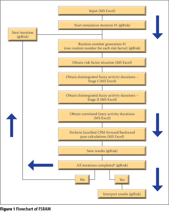
Fuzzy values obtained at the end of a simulation reveal some important project aspects, such as a possibility range of project completion duration, criticality degree of activities, path total float variations, path criticality degrees, path sensitivities to risk factors, and project sensitivities to risk factors. The flowchart that shows how FSRAM operates is illustrated in Figure 1. If more than one activity is a candidate to be influenced by the same risk factors in a schedule, the duration of these activities would be correlated. For example, if the duration of one of the two correlated activities occurred as more than expected due to risk factors during an iteration case, the duration of the other activity should also be taken as more than expected during this iteration. If such correlation effects were not incorporated into a scheduling model, unrealistic results would be obtained. Therefore, the main argument and target of FSRAM is to model the uncertain construction conditions more realistically from the scheduling point of view.

 

 

Features and operation details of FSRAM

This section presents detailed information about the operation of FSRAM under different headings that also disclose its different features.

Simplified input data

FSRAM is designed such that required input data is extremely easy to obtain. In other words, data that should be entered into FSRAM is mainly subjective, qualitative, depending on past experience, and therefore flexible for adaptation to specific conditions. The input data items that FSRAM requires are as follows:

■ Network data: Work breakdown structure, predecessor relationships between activities (finish to start, start to start, start to finish, or finish to finish) and lag/ lead times.

■ Minimum, most likely and maximum activity durations.

■ Most important risk factors that are expected to affect the schedule.

■ Activity risk factor influence degrees: These are represented in qualitative terms such as very effective, effective or ineffective. The user selects the appropriate qualification for each "activity risk factor" pair. This data shows the relative degree of how much a particular risk factor creates uncertainty on the duration of a particular activity.

■ Risk factor situation probability boundaries: In real life, risk factors may occur as better than expected, expected or worse than expected. In each situation they respectively create favourable, neutral or adverse uncertainty over activity durations. FSRAM needs to know the probability boundaries of risk factors' different situations to decide which situation will occur for a particular simulation step, so that the total effect of risk factors on activity durations is determined by the utilisation of "activity risk factor influence degrees" in conjunction with risk factor situations. "Risk factor situation probability boundaries" are judgementally determined through past experience, and entered as numerical values between 0 and 1. For instance, when the user estimates that the labour productivity risk is very probable to occur as worse than expected, less probable to occur than expected, and least probable to occur as better than expected, the user may enter 0.10-0.401.00 values respectively to represent better than expected, expected and worse than expected risk factor situation probability boundaries of this risk factor. In such a case, the probability of occurrence of better than expected, expected and worse than expected in any FSRAM iteration becomes 0.10 (0.10-0.00), 0.30 (0.40-0.10), and 0.60 (1.00-0.40) respectively.

■ Correlation between risk factors: FSRAM requires the information regarding which risk factors are correlated. For instance, if the user estimates that, as weather conditions become worse than expected, labour productivity will be worse than expected, or as weather conditions become better than expected, labour productivity will be better than expected, then he/she may introduce these risk factors to the model as correlated. Eventually, FSRAM's computation algorithm behaves accordingly.

■ Simulation properties: The user should enter the characteristic preferences for the implementation of MCS, such as the iteration number.

Elicitation of correlation between activity durations

FSRAM is eligible for indirectly eliciting correlation between activity durations. The user is not required to enter the correlation coefficients directly. Instead, correlation is supplied by activity risk factor influence degrees entered by the user in the form of very effective-effective-ineffective qualitative terms. Correlation between activity durations is captured by entering the same or close qualitative estimates (very effective-very effective for full correlation or very effective-effective for partial correlation) for any two activities thought to be sensitive to a particular risk factor.

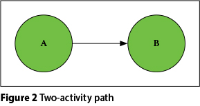
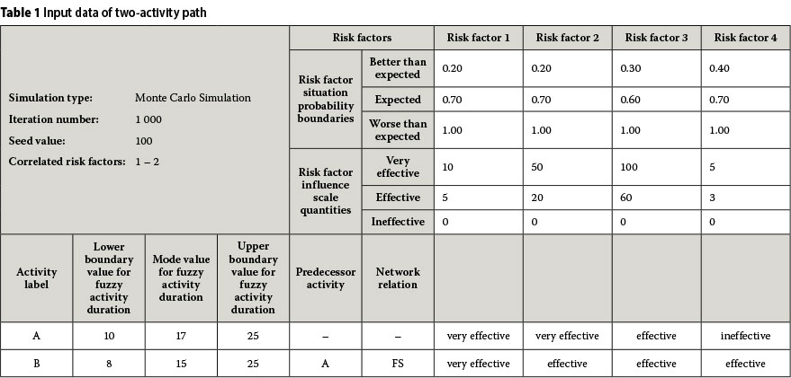
For the sake of comprehension of FSRAM's correlation capturing mechanism, consider the activity path shown in Figure 2. This path consists of two activities depending on each other. The data used in this example is presented in Table 1. Risk factor 1 and Risk factor 2 are assumed to be correlated. As shown in Table 1, both of the activities are strongly correlated when Risk factor 1 is considered, because the "risk factor - activity" degrees of influence of both activities are qualified by the very effective term. When Risk factor 3 is considered, these two activities are assumed to be correlated again by the very effective-effective pair, but weaker with respect to Risk factor 1. When Risk factor 4 is considered, they are not correlated, because Risk factor 4 is not effective in Activity A.

 

 

Now consider the iteration #1. Assume that FSRAM produced the random numbers 0.15, 0.15, 0.75 and 0.85 for risk factor i (i=1→4) respectively, in order to determine the risk factor situations for this particular iteration. FSRAM conducts this operation as follows (refer to Figure 1 and Table 1):

■ iteration #1-rnd.no.#1 = 0.15 < 0.20 better than expected (Risk factor 1)

■ iteration #1-rnd.no.#2 = 0.15 < 0.20 better than expected (Risk factor 2)

■ iteration #1-rnd.no.#3 = 0.75 > 0.60 worse than expected (Risk factor 3)

■ iteration #1-rnd.no.#4 = 0.85 > 0.70 worse than expected (Risk factor 4)

Random numbers generated for Risk factor 1 and Risk factor 2 are equal because they are assumed to be correlated. Furthermore, risk factor situation probability boundary values are the same for these two correlated risk factors. This approach enables the elicitation of the correlation between risk factors indirectly.

The procedure that FSRAM follows to compute the fuzzy activity duration of Activity A to be used in iteration #1, is described below. The description should be followed by referring to Figure 1 and Table 1. FSRAM computes all the activity fuzzy durations during simulation in the same manner so that it utilises these randomly produced fuzzy durations in fuzzy CPM calculations through subsequent iterations.

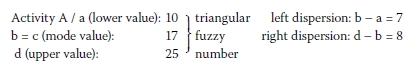
Left and right dispersion of the fuzzy duration of Activity A given in Table 1 is distributed to the risk factors in proportions with the risk factor influence scale quantity values:

left dispersion: K (10 + 50 + 60 + 0) = 7 K = 7/120

                     Risk factor 1: 7/120 x 10 = 7/12

                     Risk factor 2: 7/120 x 50 = 35/12

                     Risk factor 3: 7/120 x 60 = 42/12

                     Risk factor 4: 7/120 x 0 = 0

right dispersion: K (10 + 50 + 60 + 0) = 8 K = 8/120

                     Risk factor 1: 8/120 x 10 = 8/12

                     Risk factor 2: 8/120 x 50 = 40/12

                     Risk factor 3: 8/120 x 60 = 48/12

                     Risk factor 4: 8/120 x 0 = 0

Disintegration I (Disintegrated Fuzzy Activity Durations - Stage I):

■ Risk factor 1: (17-7/12, 17, 17 + 8/12) (16.41, 17.00, 17.67)

■ Risk factor 2: (17-35/12, 17, 17 + 40/12) (14.08, 17.00, 20.33)

■ Risk factor 3: (17-42/12, 17, 17 + 48/12) (13.50, 17.00, 21.00)

■ Risk factor 4: (17-0, 17, 17 + 0) (17.00, 17.00, 17.00)

Notice that left and right dispersions are performed by using the risk factor influence scale values in accordance with the risk factor influence degrees. This provides relative dispersion according to the influence of each risk factor. For instance, very-effective influence scale is 10 and 50 for Risk factor 1 and Risk factor 2 respectively. Since Risk factor 1 and Risk factor 2 affect Activity A with the very-effective degree, the values 10 and 50 (given in Table 1) are utilised. Furthermore, the effect of Risk factor 1 is less than the effect of Risk factor 2, because 10 is less than 50. This procedure provides the projection of the relative uncertainty effect of the risk factors on the activities.

Disintegration II (Disintegrated Fuzzy Activity Durations - Stage II):

■ Risk factor 1:

better-than-expected → 17 - [0.7 (17 - 16.41)] = 16.59

worse-than-expected → 17 + [0.7 (17.67 - 17)] = 17.47

fuzzy better-than-expected → 16.59 - 16.41 = 0.18

                                                               → (16.59 - 0.18, 16.59, 16.59 + 0.18)

                                                               → (16.41, 16.59, 16.77)

fuzzy worse-than-expected → 17.67 - 17.47 = 0.2

                                                               → (17.67 - 2 0.2, 17.67 - 0.2, 17.67)

                                                               → (17.27, 17.47, 17.67)

fuzzy expected                  → (16.77, 17, 17.27)

Notice that 0.7 (very-effective limit value) is utilised in Disintegration II, because Risk factor 1's influence degree on Activity A is very-effective and 0.7 is the limit value assigned as default by FSRAM for the very-effective influence. Effective limit value is assigned as 0.3. It is a less than very-effective limit value. This is meaningful. In Disintegration I the uncertainty in fuzzy durations entered by the user is dispersed between risk factors according to risk factor influence degrees and scales. In Disintegration II, disintegrated fuzzy durations are further dispersed to represent risk factor situations (better-than-expected, expected, worse-than-expected). If the influence of a particular risk factor is very-effective then its dispersion effect is higher (scale is 0.7); if its influence is effective then its dispersion effect is less (scale is 0.3).

■ Risk factor 2:

better-than-expected → 7 - [0.7 (17 - 14.08)] = 14.96

worse-than-expected → 17 + [0.7 (20.33 - 17)] = 19.33

fuzzy better-than-expected → 14.96 - 14.08 = 0.88

→ (14.96 - 0.88, 14.96, 14.96 + 0.88)

→ (14.08, 14.96, 15.84)

fuzzy worse-than-expected → 20.33 - 19.33 = 1.0

→ (20.33 - 21.0, 20.33 - 1.0, 20.33)

→ (18.33, 19.33, 20.33)

fuzzy expected → (15.84, 17, 18.33)

■ Risk factor 3:

better-than-expected → 17 - [0.3 (17 - 13.50)] = 15.9

5 worse-than-expected → 17 + [0.3 (21 - 17)] = 18.2

fuzzy better-than-expected → 15.95 - 13.50 = 2.45

→ (15.95 - 2.45, 15.95, 15.95 + 2.45)

→ (13.50, 15.95, 18.4 > 17)

→ (13.50, 15.95, 17)

fuzzy worse-than-expected → 21 - 18.2 = 2.8

→ (21 - 2 2.8, 21 - 2.8, 21)

→ (15.4 < 17, 18.2, 21)

→ (17, 18.2, 21)

fuzzy expected → (17, 17, 17)

■ Risk factor 4:

ineffective → (17, 17, 17)

Fuzzy duration of Activity A at the end of iteration #1:

■ Risk factor 1: better-than-expected (16.41, 16.59, 16.77)

■ Risk factor 2: better-than-expected (14.08, 14.96, 15.84)

■ Risk factor 3: worse-than-expected (17, 18.2, 21)

■ Risk factor 4: worse-than-expected (17, 17, 17)

■ Lower value (a) → 17 - 16.41 = 0.59 (-)

→ 17 - 14.08 = 2.92 (-) Total: 3.51 (-)

→ 17 - 17 = 0 a = 17 - 3.51

→ 17 - 17 = 0 = 13.49

■ Mode value (b) → 17 - 16.59 = 0.41 (-)

→ 17 - 14.96 = 2.04 (-) Total: 1.25 (-)

→ 17 - 18.2 = 1.2 (+) b = 17 - 1.25

→ 17 - 17 = 0 = 14.87

■ Upper value (d) → 17 - 16.77 = 0.23 (-)

→ 17 - 15.84 = 1.16 (-) Total: 2.61(+)

→ 17 - 21 = 4 (+) d = 17 + 2.61

→ 17 - 17 = 0 = 19.61

Then, fuzzy duration of Activity A for iteration #1 = (13.49, 14.87, 19.61)

The calculations above show that FSRAM accepts the fuzzy activity duration entered by the user as a duration interval containing all the possible outcomes of duration. Moving from this point, in each iteration it tries to find the realistic fuzzy duration that lies on this interval, according to the risk factor situations determined randomly. In order to perform this process, it follows the risk factor based and correlated calculation algorithm described above. FSRAM takes the mode values of the fuzzy durations entered by the user as a standpoint, disperses the total risk factor effect around this point and finally finds out the fuzzy activity durations in any iteration.

Evaluation of uncertainty in project duration

FSRAM calculates different fuzzy durations for the activities in each iteration case during MCS (refer to Figure 1). Then it performs fuzzy forward-backward pass CPM calculations by using these fuzzy durations. At the end of each iteration, a different fuzzy project duration is calculated. The problem here is how to evaluate all of these fuzzy durations and make inferences about the uncertainty effect of the project completion time. FSRAM solves this problem by using the lower, upper and mode values of the fuzzy project durations found through simulation. It finds the mean of the mode values, minimum of the lower values and maximum of the upper values, and assigns these respectively as the mode, lower and upper values of the final fuzzy project duration. Table 2 contains the simulation results for lower (a), mode (b = c) and upper (d) values of 20 iterations of FSRAM on a network containing seven activities and the calculation of the final fuzzy project duration. Figure 3 shows the fuzzy project duration in diagrammatic form.

 

 

 

 

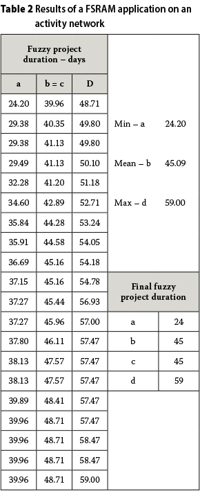
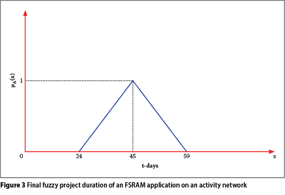
When Table 2 and Figure 3 are examined, it can be seen that 45 days have the greatest possibility for being the duration of the project, because its membership degree is 1.0. However, the project duration might be between 24 and 59 days; the duration values decrease as they get further away from 45 and approach either 24 or 59 days.

Assessment of activity and path criticalness

The uncertainty in criticalness of activities and paths of a network is another problematic issue for which FSRAM offers solutions. In traditional CPM, the criticalness of an activity is simply determined by checking the total float time of the activity. However, in a simulation-based method like FSRAM, early start, early finish, late start and late finish times, and in turn, total float times of activities are obtained different from one another in any simulation iteration.

If the activity fuzzy early and fuzzy late times are converted to single crisp characteristic values, then the total float time of an activity can be approximately calculated. The best way for this is to use the duration values corresponding to the geometric centre of the trapezoidal fuzzy numbers.

Total float time in traditional CPM is found by Equation 1.

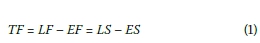
where LF, EF, LS and ES designate late finish, early finish, late start and early start times of an activity respectively.

Since LF, EF, LS and ES are all in fuzzy numbers in FSRAM, geometric centres of these fuzzy numbers (calculated by Equation 2) can be used to find the total float time of any activity x Є X (the set of activities) approximately:

where C designation denotes the geometric centre of the early and late times.

FSRAM finds different total float times for the activities during simulation. This means that the criticalness of each activity changes. In turn, the criticalness of paths changes. The float time of a path is an indication of the path criticalness. Path float times can be found by summing up the total float times of the activities on a path. If the total float time of a path is calculated as zero or approximately zero, then it can be concluded that this path is the critical path. Near critical and uncritical paths can also be explored by examining the path float times.

Elicitation of correlation between risk factors

Another distinguishing feature of FSRAM is its capability of modelling the correlation between risk factors. The indirect elicitation method is followed just as it was for the correlation elicitation between activities. In other words, correlation coefficients between risk factors are not required. Risk factors are not represented with probability distributions in FSRAM; accordingly, correlation coefficient values are not necessary, but instead are represented by risk factor situation probability boundaries. This input data is requested from the user in quantitative terms between 0 and 1, based on engineering judgement, experience and historical data. FSRAM provides the correlation between risk factors through two steps - firstly it equates the risk factor situation probability boundaries of the risk factors that the user has entered into the model as correlated, and secondly it generates the same random numbers for the correlated risk factors to determine their risk factor situations and to compute the durations of the activities that are affected by them. The activity duration computation procedure is the same as shown in the previous section.

Simulation-based uncertainty evaluation algorithm

FSRAM evaluates the uncertainty in a construction schedule network by executing the MCS technique. Scheduling is a complex problem, and a model produced for analysing a schedule cannot be solved analytically. Simulation techniques are utilisable in such cases.

Activity-, path-, and project-based risk factor sensitivity analysis

FSRAM is capable of detecting which risk factors are more effective for each activity, for each path and for the project duration. It performs this by executing the simulation for each risk factor one at a time, and comparing the change in activity, path float times and project duration. By this way FSRAM provides useful information to a manager or decision-maker about the uncertainty inherent in a construction project.

 

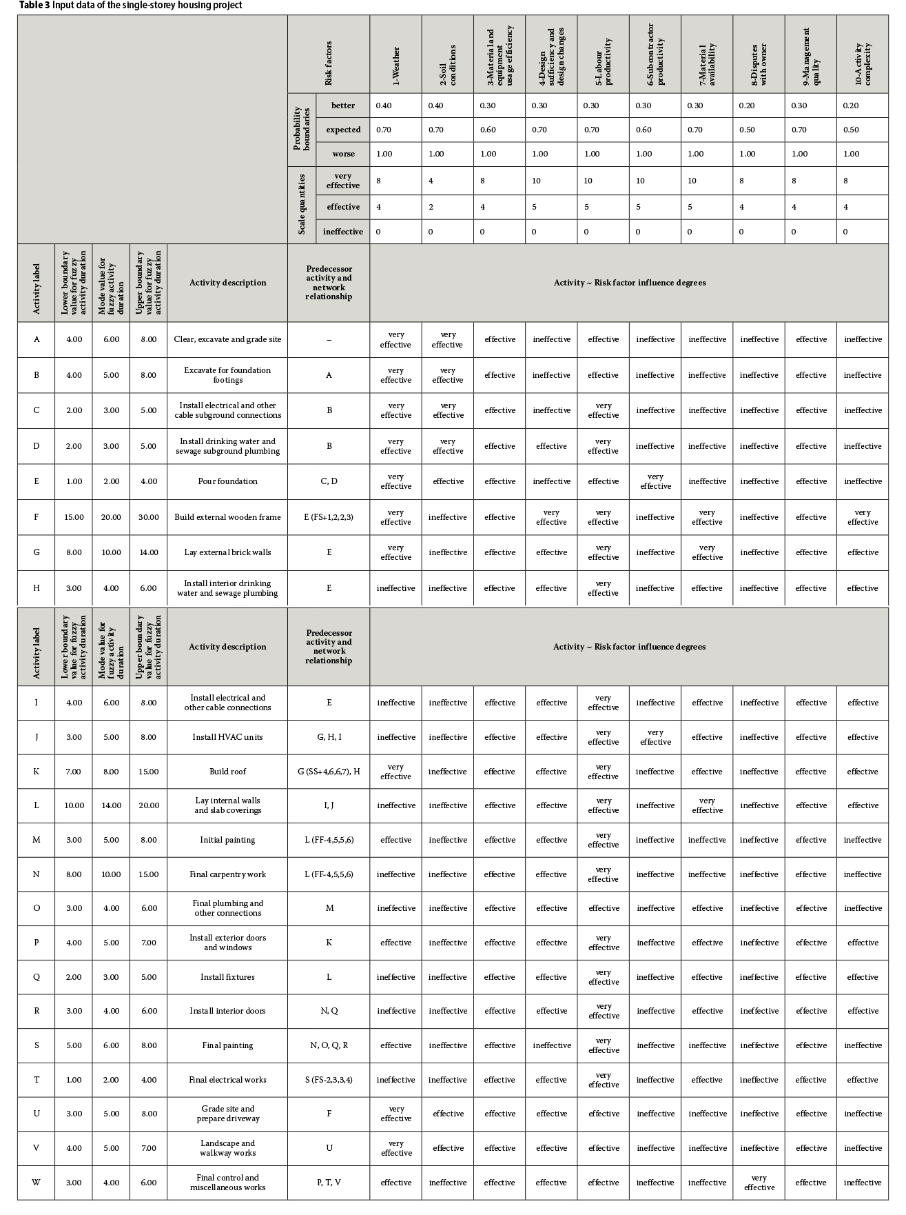
AN EXAMPLE FSRAM APPLICATION

In this section FSRAM is being evaluated on a single-storey housing project. Input data of the project is given in Table 3. Ten risk factors are assumed to influence the schedule - Risk factor 1 and Risk factor 2, Risk factor 7 and Risk factor 9, Risk factor 8 and Risk factor 10 are assumed to be correlated. The results of FSRAM application are also compared with the results of CPM and MCS-based CPM applications.

MS Excel and @Risk software programs have been used for the model's execution. In Figure 1 the utilised software in each step is mentioned next to each item of the model's operation flow chart. @Risk is indeed an add-in of MS Excel. It adds risk analysis and simulation capability to MS Excel. After any simulation it reports the statistical results automatically in a regulated fashion. In this regard the results of the FSRAM execution that are introduced through the next sections have been extracted from @Risk's reports, and summarised. The application of MCS-based CPM has also been performed by using both MS Excel formulae and @Risk.

Application of CPM, MCS-based CPM and FSRAM on the project

CPM, MCS-based CPM and FSRAM have been applied on the project data given in Table 3. Only the required parts of the data given in Table 3 have been used in these independent applications. For instance, mode values of fuzzy activity durations have been used as the activity durations in CPM application. Furthermore, the lower, upper and mode values of fuzzy activity durations have been used to assign triangle probability distributions to the activity durations in MCS-based CPM application. However, in FSRAM application, all the data given in Table 3 has been utilised.

The correlation effect between the activity durations, the correlation coefficients captured and the final fuzzy project durations have been observed and compared at the end of applications. In MCS-based CPM and FSRAM applications, 1 000 MCS iterations were conducted. It is assumed that correlation coefficients are not known in advance and, depending on this, all the risk factors have been assumed as uncorrelated in MCS-based CPM application.

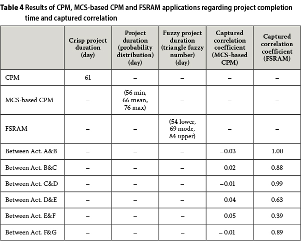
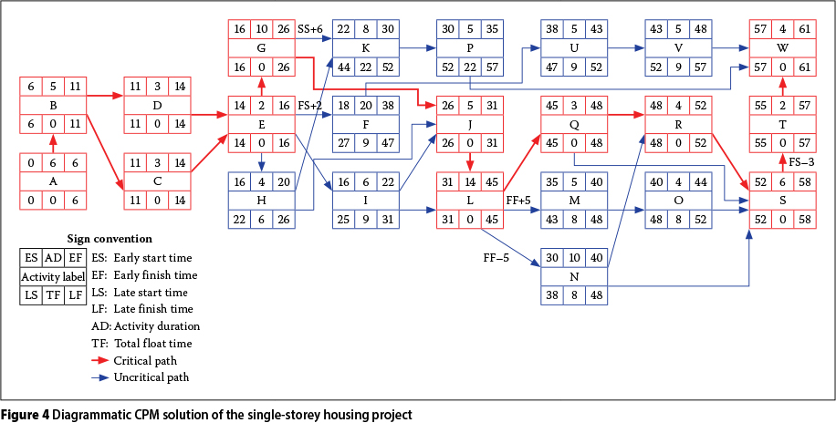
Table 4 contains the results of the CPM, MCS-based CPM and FSRAM applications. Furthermore, a CPM solution is illustrated with an activity-on-node network diagram in Figure 4. The results show that the minimum and maximum project durations found by MCS-based CPM, which are 56 and 76, are different from the lower (a) and upper (d) fuzzy project duration values found by FSRAM, which are 54 and 84. In other words, the uncertainty range produced by MCS-based CPM (which is 76 - 56 = 20) is lower than the uncertainty range produced by FSRAM (which is 84 - 54 = 30). FSRAM reflects the uncertainty effect on the project completion time realistically, because it follows a risk-based simulation methodology and takes the correlation effect between activities and between risk factors into account. In contrast, MCS-based CPM is not risk-based and it does not take the correlation effect into account. Therefore, the result produced by FSRAM regarding the uncertainty of project duration is more reliable. Table 4 and Figure 4 show that the project duration is 61 days according to CPM. This is already a crisp value and does not give any idea about uncertainty. Furthermore, "61 days" is very close to the lower duration value of FSRAM, which is 54 days. This means that schedule overrun would be highly possible if the decisions regarding the project duration were taken by using CPM.

The results given in Table 4 reveal that the correlation coefficients captured by FSRAM between the activities A-B, B-C, C-D, D-E, E-F and F-G are 1.00, 0.88, 0.99, 0.63, 0.39, and 0.89 respectively. This shows that the model produces realistic results in capturing correlation indirectly between activity durations and risk factors. For instance, the correlation coefficient found for Activities A and B, which is the highest, is logical because all the influence degrees assigned to these activities are the same as shown in Table 3. The correlation coefficient found for Activities E and F, which is the lowest, is logical because most of the influence degrees assigned to these activities are different. The correlation coefficients captured by MCS-based CPM between the activities A-B, B-C, C-D, D-E, E-F and F-G are all close to zero, as given in Table 4. This is expected because MCS-based CPM is not able to take the correlation effect into account.

Risk factor sensitivity analysis

As previously mentioned, it is also possible to conduct sensitivity analysis with FSRAM. Knowing which risk factors are more effective on the project and on the paths gives the manager the opportunity of managing the schedule better.

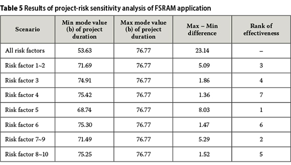
Table 5 contains the results of the project-risk sensitivity analysis. When the results are examined, it is observed that Risk factor 5 (labour productivity) creates the greatest maximum-minimum difference with respect to the mode value (b) of project duration. This means that Risk factor 5 is more responsible for the project duration uncertainty. Furthermore, the other maximum-minimum difference values with respect to the mode value (b) of project duration in Table 5 reveal that Risk factor 1 ~ Risk factor 2 (weather ~ soil conditions) and Risk factor 7 ~ Risk factor 9 (material availability ~ management quality), which are correlated in-between, are the other most effective risks after Risk factor 5. It is important to focus on these risk factors during the management of the project. However, the risk factors which are more effective, especially on the uncritical paths that are the candidates for turning to critical due to the uncertainty effect, should also be known in advance to manage the paths properly and decrease the uncertainty effect.

 

 

FSRAM computes the float times of the paths by subtracting the sum of durations of activities on a path from the project duration during simulation iterations. FSRAM has detected 34 paths in the network of the example housing project. Table 6 contains the results of the first portion of the path-risk sensitivity analysis. The results given in Table 6 reveal that some of the paths show more variability with respect to their float times. Possible minimum and maximum float values are an indication of this variability. For instance, consider paths 4 and 11. Path 4 is an uncritical path according to CPM. However, FSRAM finds that its float time may change from 3.88 days to 14.97 days, which means that its un-criticalness is highly uncertain. Path 11 is also an uncritical path according to CPM. However, FSRAM finds that its float time may change from 3.81 days to 5.35 days, which means that it is a near critical path. Then, knowing which risk factors are more effective on such paths is important for a manager to take precautions in advance to prevent these paths from becoming critical. Besides the uncritical paths of CPM, critical paths are also important for focusing attention. Consider path 1 and path 2 in Table 6. They are critical paths according to CPM. Therefore, they have no opportunity to extend in duration. If they extend, the project duration would extend. Since the critical paths have zero float times, they are difficult to manage, because any extension of such paths directly leads to the extension of the project duration.

 

 

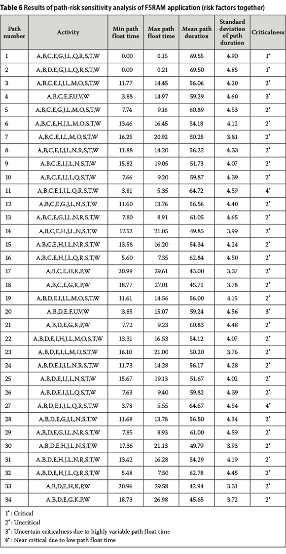
Table 6 and Table 7 contain the results that FSRAM has produced about which paths are highly uncertain in criticalness, and which risk factors are mostly responsible for this uncertainty. FSRAM performs such an analysis in two steps: by running the risk factors all together first and then running them separately.

The results in Table 7 show that Risk factor 5 (labour productivity) is the risk most responsible for the uncertainty in path durations. It stands in the first order of the most affecting risk factors for almost all of the paths. Furthermore, Risk factor 1 ~ Risk factor 2 (weather ~ soil conditions) and Risk factor 7 ~ Risk factor 9 (material availability ~ management quality), which are correlated in-between, are the other most effective risks after Risk factor 5. This is compatible with the result obtained in project-risk sensitivity analysis. In other words, these three risk factors are the most effective factors, not only with regard to path duration uncertainty, but also as far as project duration uncertainty is concerned.

Paths 1, 2, 4, 11, 17, 18, 20, 27, 33 and 34 are the paths on which the managerial attention should be focused first for the sake of project success, because they are either critical, near critical, uncertain critical or uncritical.

 

LIMITATIONS OF FSRAM

FSRAM has some limitations, as briefly described below:

■ Dependence on realistic input data: In order to get realistic results from FSRAM, the data entered to the model should be realistic.

■ Default model parameters: Activity ~ risk factor influence degrees are entered as either very-effective, effective or ineffective qualitative terms. However, one may argue about very-very-effective or very-very-very-effective terms.

■ Ignorance of implication dates and location of activities: An activity that is affected extremely by a particular risk factor during certain periods of the year may not be affected by the same risk factor in different time periods (weather-sensitive activities are good examples). Or, an activity that is affected extremely by a particular risk factor in certain locations of a construction site may not be affected from the same risk factor in different locations of the same site. FSRAM is not capable of modelling such marginal situations.

 

CONCLUSIONS AND FUTURE WORK

In this paper, a new schedule risk analysis model called FSRAM has been introduced. FSRAM is a simulation-based model developed for the purpose of evaluating construction activity networks under uncertainty when activity durations and risk factors are correlated. The operational logic of the model and an example FSRAM application of a housing project are included in the paper. The results of the FSRAM application show that FSRAM operates well and produces realistic results regarding the uncertainty extent inherent in the schedule. However, this conclusion cannot be generalised. FSRAM should be tested on several schedules of different types of civil engineering projects for full evaluation. Further case studies are being carried out for this purpose; this paper comprises only the development of the model. FSRAM can be computerised easily by utilising table processor software and embedded macros, and can be further designed in a user-friendly form. In this paper, MS Excel and @Risk software programs have been used for FSRAM's execution. A superior computerised form of it can be proposed as a future task.

 

REFERENCES

Ahuja, H N & Nandakumar, V 1985. Simulation model to forecast project completion time. Journal of Construction Engineering and Management, 111(4): 325-342.         [ Links ]

Ang, A H, Chaher, A A & Abdelnour, J 1975. Analysis of activity networks under uncertainty. Journal of Engineering Mechanics Division, 101(4): 373-387.         [ Links ]

Carr, R I 1979. Simulation of construction project duration. Journal of Construction Division, 105(2): 117-128.         [ Links ]

Chao, L C 20 07. Fuzzy logic model for determining minimum bid mark-up. Computer-aided Civil and Infrastructure Engineering, 22(6): 449-460.         [ Links ]

Department of the Navy 1958. PERT, program evaluation research task. Washington: Phase I Summary Rep, Special Projects Office, Bureau of Ordnance.         [ Links ]

Diaz, C F & Hadipriono, F C 1993. Nondeterministic networking methods. Journal of Construction Engineering and Management, 119(1): 40-57.         [ Links ]

Edwards, L 1995. Practical risk management in the construction industry. London: Thomas Telford.         [ Links ]

Flanagan, R & Norman, G 1993. Risk management and construction. Cambridge: Backwell Scientific.         [ Links ]

Griffis, F H & Farr, J V 2000. Construction planningfor engineers. Singapore: McGraw-Hill.         [ Links ]

Halphin, D W & Woodhead, R W 1998. Construction management. New York: Wiley.         [ Links ]

Jaafari, A 1984. Criticism of CPM for project planning analysis. Journal of Construction Engineering and Management, 110(2): 222-223.         [ Links ]

Jin, X L & Doloi, H 2009. Modelling risk allocation decision-making in PPP projects using fuzzy logic. Computer-aided Civil and Infrastructure Engineering, 24(7): 509-524.         [ Links ]

Levitt, R E & Kunz, J C 1985. Using knowledge of construction and project management for automated schedule updating. Project Management Journal, 16(5): 57-76.         [ Links ]

Oberlender, G D 200 0. Project management for engineering and construction. Boston: McGraw-Hill.         [ Links ]

Ökmen, Ö & Öztaş, A 2008. Construction project network evaluation with correlated schedule risk analysis model. Journal of Construction Engineering and Management, 134(1): 49-63.         [ Links ]

Öztaş, A & Ökmen, Ö 2005. Judgmental risk analysis process development in construction projects. Building and Environment, 40(9): 1244-1254.         [ Links ]

Ranasinghe, M & Russell, A D 1992. Treatment of correlation for risk analysis of engineering projects. Civil Engineering Systems, 9(1): 17-39.         [ Links ]

Sadeghi, N, Fayek, A R & Pedrycz, W 2010. Fuzzy Monte Carlo simulation and risk assessment in construction. Computer-aided Civil and Infrastructure Engineering, 25(4): 238-252.         [ Links ]

Stathopoulos, A, Dimitriou, L, & Tsekeris, T 2008. Fuzzy modelling approach for combined forecasting of urban traffic flow. Computer-aided Civil and Infrastructure Engineering, 23(7): 521-535.         [ Links ]

Touran, A & Wiser, E P 1992. Monte Carlo technique with correlated random variables. Journal of Construction Engineering and Management, 118(2): 258-272.         [ Links ]

Wang, W-C & Demsetz, L A 2000a. Application example for evaluating networks considering correlation. Journal of Construction Engineering and Management, 126(6): 467-474.         [ Links ]

Wang, W-C & Demsetz, L A 2000b. Model for evaluating networks under correlated uncertainty -NETCOR. Journal of Construction Engineering and Management, 126(6): 458-466.         [ Links ] Woolery, J C & Crandall, K C 1983. Stochastic network model for planning scheduling. Journal of Construction Engineering and Management, 109(3): 342-354.         [ Links ]

 

 

Correspondence:
Ö Ökmen
Devlet Su İşleri Genel Müdürlüğü
(General Directorate of State Hydraulic Works)
Proje ve İnşaat Dairesi Başkanlığı
Devlet Mah
İnönü Bulvarı
No: 16, 06100 Çankaya
Ankara
TURKEY
T: +90 532 288 1322
E: onderokmen@hotmail.com / onderok@dsi.gov.tr

A Öztaş
University President
Ishik University
100 Meters Avenue
Erbil
IRAQ
T: +964 66 252 9841/ +964 750 704 6969
E: ahmet.oztas@ishik.edu.iq / president@ishik.edu.iq

 

 

 

DR ÖNDER ÖKMEN is an engineer at the General Directorate of State Hydraulic Works in Turkey. He obtained his BSc degree in Civil Engineering from the Middle East Technical University, and his MSc and PhD degrees in Construction Management (Civil Engineering) from the Gaziantep University in Turkey. He did post-doctoral research at the Epoka University in Albania. Currently he is busy with irrigation and drainage projects. His research interests include project management, risk analysis, scheduling, cost estimation, irrigation channels and pipe networks.

 

 

PROF DR AHMET ÖZTAŞ. is the President of Ishik University in Erbil, Iraq. He obtained his BSc degrees in Mathematics from İnönü University and in Civil Engineering from lstanbul Technical University in Turkey, and his MSc and PhD degrees in Management from Istanbul University and in Civil Engineering from Manchester University, respectively After lecturing at the Gaziantep University for many years, he worked as faculty dean and lecturer at the Epoka University in Albania. His research interests include construction project management, expert systems, risk analysis, scheduling and cost estimation.