TECHNICAL PAPER

 

Incorporating rainfall uncertainty into catchment modelling

 

 

J G Ndiritu

Contact details

 

 

---

ABSTRACT

A framework for incorporating areal rainfall uncertainties into catchment modelling is presented and demonstrated through the daily streamflow simulation of the Mooi River catchment using the Australian Water Balance Model (AWBM). The framework is an extension of the typical hybrid manual-automatic model calibration-validation in which uncertainties are imposed as perturbations (disturbances) on the rainfall time series. The differences in areal rainfall obtained from different rain-gauge densities are used to generate the perturbations, and their variability is found to reduce as areal rainfall magnitude increases. The applied probability distributions of perturbations are therefore obtained for specified ranges of rainfall magnitude. The effect of incorporating uncertainties is assessed by finding out the impact of imposing perturbations on the validation performance of the rainfall-runoff modelling. This is done by carrying out 100 rainfall-runoff calibration-validation runs with perturbed and with unperturbed rainfall and comparing the 100 generated validation period runoff time series with the observed (historical) runoff series. With perturbations applied, the 5-95 percentile bounds from the resulting 100 streamflow ensembles contain 52% of the observed time series for the validation period. Without perturbations, only 25% of the observed flows fall within the bounds. The framework has the potential for practical use, but this would require a more rigorous identification of appropriate distributions of the perturbations.

Keywords: rainfall uncertainties, catchment modelling, multipliers, calibration

---

 

 

INTRODUCTION

Areal rainfall is recognised as a major contributor to uncertainty in catchment modelling (Kavetski et al 2006a,b; Sawunyama 2008; Hughes et al 2011), although it is not formally incorporated into hydrological analysis in southern Africa (Sawunyama 2008) and many other regions of the world. While improving rainfall measurement is considered vital for well-informed decision-making in water resources management (Hughes et al 2011), many regions of the world may not have the resources to install and maintain the required data networks (Sawunyama 2008). Even if this were possible, areal rainfall estimation for the practically installable rain-gauge density is still likely to be substantially uncertain. Remote-sensing approaches require validation using rain-gauge measurements (Sawunyama 2008) and are therefore unlikely to reduce these uncertainties to insignificant levels. The need to formally incorporate rainfall uncertainty into catchment modelling is therefore essential. Bayesian approaches have recently been applied for the incorporation of uncertainties of rainfall and other variables and have generally been assessed as effective (Kavektsi et al 2006a,b; Ajami et al 2007; Vrugt et al 2009; Kuczera et al 2006, 2010; Balin et al 2010). Their complexity and high computational requirements, however, pose serious challenges to their application in practice. Sawunyama (2008) investigated the effect of rainfall uncertainties by obtaining areal rainfalls from different rain-gauge densities (by systematically omitting some valid stations from areal rainfall estimation) and comparing the modelled streamflow sequences using these different rainfall station configurations. Rainfall uncertainty was found to be more significant for mountainous areas and the main recommendation was to improve rainfall measurement density in order to reduce uncertainty.

This paper presents an approach for incorporating rainfall uncertainties into catchment modelling within the typical hybrid manual-automatic calibration framework. The rainfall multiplier approach of quantifying uncertainty (Kavektsi et al 2006 a, b), which has been found suitable in a recent field study (McMillan et al 2011), is applied. The framework obtains the multipliers randomly from probability distributions derived from the rainfall data. The current approach also incorporates parameter uncertainty, with the prior parameter distributions taken as uniform distributions within the specified lower and upper bounds, and the posterior as the distribution of the parameter values obtained from the randomly initialised calibration runs. This is in contrast with the more complex Bayesian approaches(Kavetski et al 2006a, b) that update parameter distributions within a single computation run. The framework is assessed by the split-sample method and a control experiment in which no disturbances (multipliers) are applied. The effect of rainfall uncertainties on the optimisation effort required in calibration is assessed by comparing the validation performance obtained from two levels in rigour of optimisation.

 

METHODOLOGY

Figure 1 presents the framework for incorporating rainfall uncertainty for the common streamflow simulation problem and could be easily adapted to other catchment modelling problems (water quality, groundwater, sediment generation, etc). The areal rainfall obtained by any appropriate method (e.g. Thiessen polygons) is perturbed by multipliers obtained randomly from a probability distribution derived from the rainfall data. An areal rainfall r_t for period t thus becomes r_t x m_t, where m_t is the multiplier for period t. The number of perturbed rainfall sequences that need to be generated (ensemble size) is selected and a population of perturbed rainfall sequences is thus obtained. Each of these is used, together with other required inputs, for multiple calibrations of the model. An understanding of the model structure, the catchment characteristics, previous experience and other information is used to establish the starting parameter ranges and the parameter range limits for the calibration. Where the uncertainties regarding the realistic parameter values are large, the starting ranges will be set more widely. The ranges therefore effectively act as quantifiers of parameter uncertainty and define the prior distribution of the parameters. Depending on the purpose of the modelling, an appropriate objective function is also selected for the calibration.

 

 

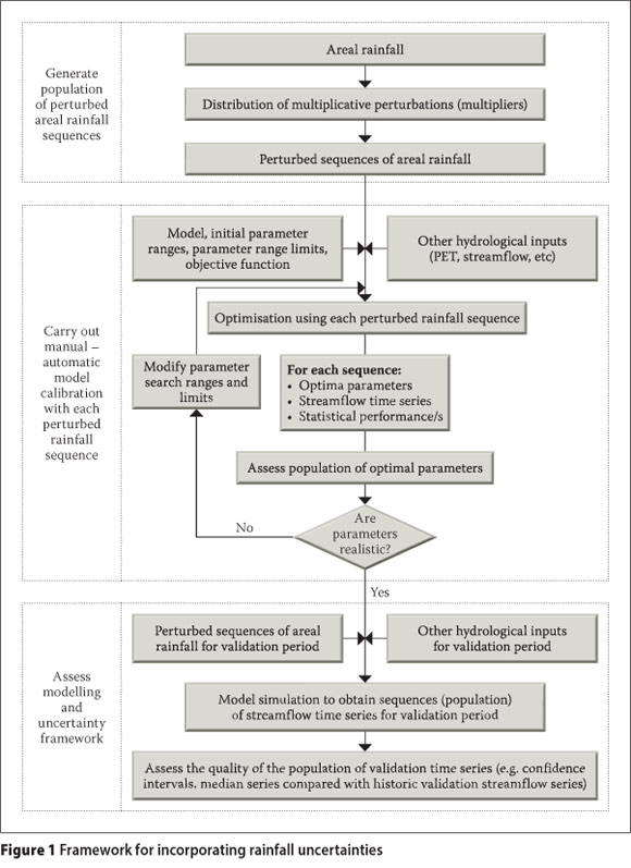
Each calibration run (for each perturbed rainfall sequence) provides an "optimal" parameter set and a population of optimal parameters is finally obtained. An assessment of this population and the calibrated streamflow time series makes it clear how realistic the modelling is and helps to identify any unexpected behaviour. This may then require adjustment of the parameter range limits and could also provide leads to aspects of significant catchment processes that were ignored or not recognised (Ndiritu 2009b). After the practically imple-mentable changes have been made (and the calibration runs repeated if need be), each of the "optimal" parameter sets is used with a perturbed rainfall series (and other required inputs) for a period that was not applied to calibrate the model. The result is a population of validation streamflow time series. A comparison between the observed validation time series and the generated population of validation streamflows shows how suitable the framework is for the specific problem.

 

APPLICATION OF FRAMEWORK

The uncertainty framework was applied to daily streamflow modelling of the Mooi River catchment in South Africa using the Australian Water Balance Model (AWBM) and multiplicative perturbations (multipliers) of rainfall derived from ratios of areal rainfall obtained from various rain-gauge densities. The widely applied SCE-UA optimiser (Duan et al 1992) was selected for calibration and maximising the coefficient of efficiency as the objective function. The ensemble (population) size was subjectively selected as 100.

The catchment

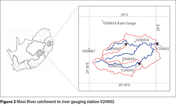
The Mooi River headwaters up to river-gauging station V2H002 were included in the analysis and were delineated into three sub-catchments: up to gauging stations V2H005 and V2H007, and the incremental area from these two to V2H002. Figure 2 shows the location of the catchment in South Africa, the three sub-catchments and the four rain-gauging stations used to obtain areal rainfall. Daily evaporation measurements were obtained from station V7E003A located outside the catchment. Flow and evaporation data were obtained from the Department of Water Affairs' (DWA) website (http://www.dwa.gov.za/hydrology), while rainfall was obtained from a rainfall database and extraction facility (Lynch 2003; Kunz 2009). The period 3 November 1973 to 19 August 1976 was used for calibration and that from 20 August 1976 to 7 June 1979 for validation. The selection was based on the need to have a continuous dataset with minimal human impacts.

 

 

The catchment model

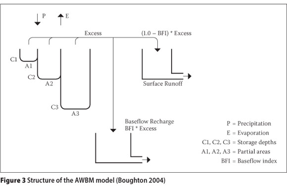
The AWBM model (Boughton 2004) is widely used for daily rainfall-runoff modelling in Australia and for flood hydrograph prediction when applied in hourly time steps. An approach for estimating runoff for ungauged catchments in Australia using the AWBM model has also been developed (Boughton & Chiew 2007). Makungo et al (2010) applied the AWBM to the Nzhelele catchment of Limpopo Province, South Africa. The AWBM was selected on the basis of its robust structure and successful application. The ACRU model (Schulze 1989) is widely applied for daily catchment modelling in South Africa, but is data-intensive and has not been set up for hybrid manual-automatic calibration. ACRU was therefore not an optimal choice for this study, although it is possible to adapt the rainfall uncertainty framework for application with ACRU. The AWBM model (Figure 3) assumes that the catchment consists of three stores of different depths C1, C2 and C3 which respectively occupy different proportions of the catchment, indicated as partial areas A1, A2 and A3 in Figure 3. At each time period, runoff is generated as the sum of the excess (overflow) from each store. The runoff is then divided into surface runoff and baseflow in proportions determined by the baseflow index (BFI). The surface runoff and the baseflow at the catchment outlet are each subjected to linear attenuation and are then summed to give the flow at the catchment outlet. Boughton (2004) provides more details of the AWBM model.

 

 

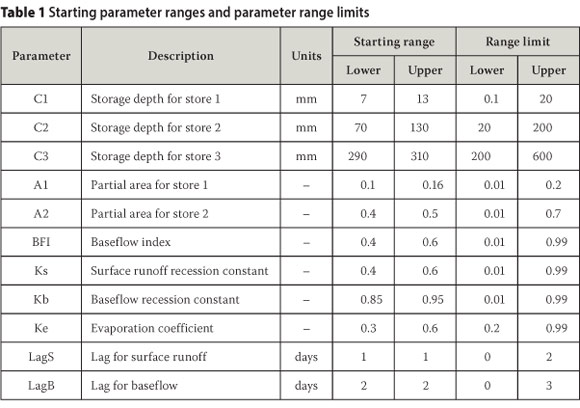
The model applied in this study also included lags for both surface runoff and baseflow, and a coefficient for scaling open-water evaporation to effective catchment evapotranspiration, giving a total of 12 parameters for each sub-catchment. The partial areas A1, A2 and A3 are expressed as proportions of the total area and therefore sum to unity. Only two of the three therefore need to be calibrated and 11 parameters were calibrated for each sub-catchment. These are shown in the first two columns of Table 1. Although the recession constants can be obtained directly from the data, it was decided to calibrate them, as an effective calibrator would have no difficulty obtaining these parameters for a well-structured model. Table 1 shows the starting parameter ranges and the range limits that were used in this study based on the understanding of the model structure, literature sources(Boughton 2004, Boughton & Chiew 2007) and past experience of modelling the Mooi River catchment.

 

 

Probability distribution of multiplicative perturbations

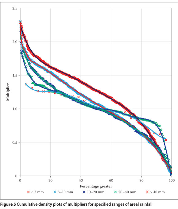
Some studies have assumed that the multiplicative perturbations (multipliers) can be obtained from a log-normal distribution(Kavetski et al 2006b; Thyer et al 2009) and this has been largely supported by an experimental study (McMillan et al 2011), although the log-normal distribution did not capture the upper-end tail of the data adequately. McMillan et al (2011) therefore proposed trials with other distributions as well. No other field data-based studies on multiplier distributions were found in the literature, and assuming that distributions fitting well in one region will do the same in another may also not be justifiable. For the current study, plausible values of multipliers were determined by computing ratios of daily areal rainfall values obtained from different rain-gauge densities for the study catchment. Thiessen polygons were used to obtain the areal rainfalls and this was confined to the days with non-zero rainfalls at all stations. It is expected that the multiplier values should depend on the magnitude of the areal rainfall as larger rainfall storms cover bigger areas and less variable rainfall would therefore be recorded at the different rain gauges. The observed variation of the multipliers with the areal rainfall (obtained at the highest rain-gauge density) is presented as Figure 4 and it reveals the expected reduction in multiplier variability as areal rainfall increases. Figure 4 also reveals that very large variations of areal rainfall could be obtained by simply omitting one or two rain gauges. It was decided to incorporate the observed reduction in multiplier variability in generating the perturbations by obtaining probability distributions for different ranges of areal rainfall magnitude. After some trial runs, the rainfall ranges selected were: < 3, 3-10, 10-20, 20-40 and > 40 mm. The multipliers within each range were ranked and plotted in order of magnitude, with the rank transformed into a percentage (non-exceedance probability), akin to the plotting of flow-duration curves. This resulted in the cumulative density plots presented in Figure 5. The multiplier to apply for a given areal rainfall was then randomly obtained from the respective probability distribution, based on the rainfall magnitude.

 

 

 

 

Experimental set-up

In order to evaluate the impact of incorporating rainfall perturbations, a control experiment consisting of 100 randomly initialised calibrations of the catchment with the unperturbed rainfall data was included. It was also decided to assess the effect of incorporating uncertainties on the required level of optimisation for calibration because it was considered likely that perturbing data could reduce the effectiveness and therefore the need for high levels of optimisation. The optimiser selected for this study, the SCE-UA (Duan et al 1992), is widely used and has been found to be effective and efficient (Ndiritu 2009a). The SCE-UA generates a population of solutions (parameter values) and divides these into a number of complexes. Each complex evolves independently, using the downhill simplex method for a set number of evolutions. The complexes are then shuffled to exchange valuable information among them and a new set of independent evolutions (epoch) commences. This process repeats until the set convergence criteria are achieved. The default SCE-UA optimisation parameters as specified by Duan et al (1994) were applied here and the level of optimisation was varied by setting the two parameters that Duan et al (1994) did not specify, namely the number of complexes to use and the convergence criterion to apply. The higher optimisation level applied 10 complexes and the convergence criterion was specified as an improvement of less than 10% in the best solution (objective function value) of the current epoch in comparison with the best solution from the epoch two steps before (the one before the previous epoch). For the lower optimisation level, five complexes were applied and convergence was specified as an improvement of less than 10% in the best solution from the current epoch in comparison with the best one from the previous epoch.

A set of 100 calibration runs with and without perturbations was therefore carried out at the higher and the lower levels of optimisation. The analysis reported in the next section thus compares results from the following four experiments: (i) higher optimisation effort with perturbations; (ii) higher optimisation effort with no perturbations; (iii) lower optimisation effort with perturbations; and (iv) lower optimisation effort with no perturbations. The lower level took 110 minutes (on a standard desktop PC), while the higher level of optimisation took 11 hours (six times longer).

 

RESULTS AND DISCUSSION

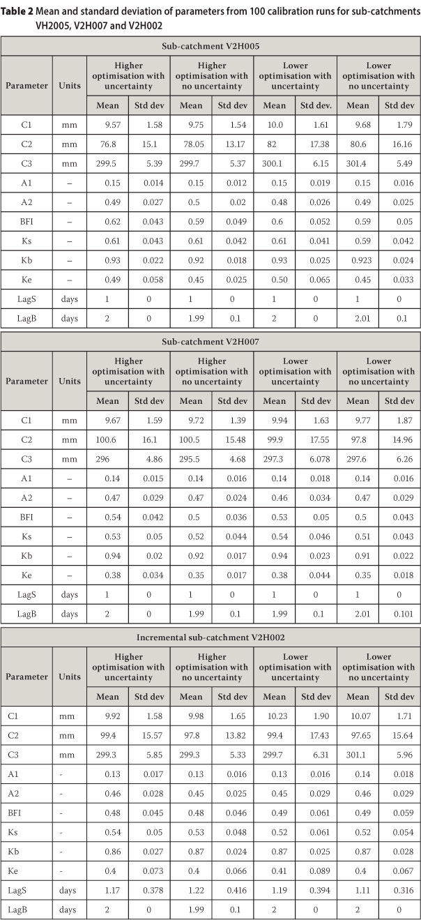
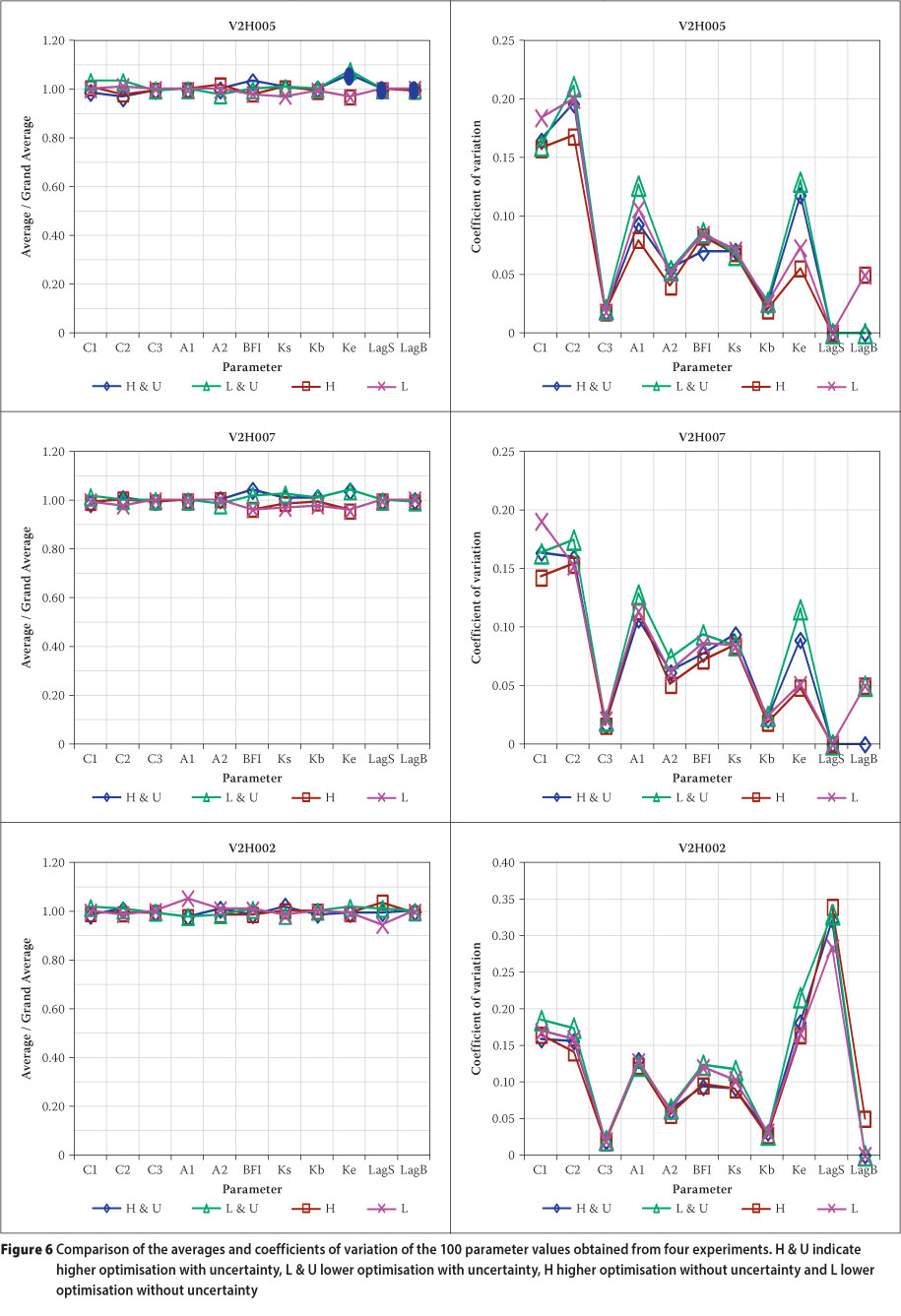
Table 2 provides the mean and standard deviations of the 100 values obtained for the three sub-catchments. All the parameter values were found to be realistic. The mean parameter values from the four experiments are very close and mostly within 95-105% of the grand average (average parameter from all four experiments), as seen in Figure 6. Figure 6 also presents plots of the coefficients of variation (mean/standard deviation) of the parameters. It is observed that the coefficients of variation of only the evaporation coefficient (Ke) consistently increase with the inclusion of rainfall uncertainties. This happens for sub-catchment V2H005 and V2H007 but not for V2H002. The mean and coefficient of variation for the surface lag (LagS) is also notably higher for V2H002 than for the other sub-catchments and a probable explanation for these differences is offered later in this section. The effect of rainfall uncertainty on parameter Ke could be attributed to the direct impact of perturbations on rainfall on the computed net rainfall (rainfall - Ke x evaporation). The observed dependence of only one parameter on rainfall uncertainty is consistent with the finding by Kuczera et al (2006) who found that only two out of the seven parameters of the LogSPM model were dependent on rainfall uncertainty.

Figure 7 shows the probability density plots and normal distribution fits for parameters Ke and A2 for sub-catchment V2H005. Although the differences in variability were not substantial for parameter A2, the plot in Figure 7 helps to illustrate the ability of the calibration to search for and obtain optimal parameters beyond the starting range specified in Table 1. This table specifies the starting range as 0.4-0.5 for A2, whereas a substantial proportion of the optimal parameters for A2 in Figure 7 locate beyond 0.5. From Figure 7 it is observed that applying perturbations leads to a notably larger spread in variability for parameter Ke at both optimisation levels, whereas the effect on the variability of A2 was only slight. Incorporating uncertainties shifted the location of the distribution of Ke, but the average Ke values for all four experiments were still reasonably close.

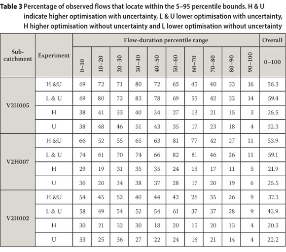
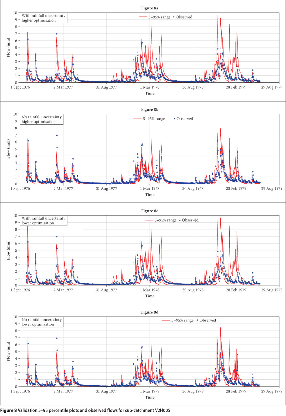
Figure 8 shows the 5-95 percentile range obtained from the 100 ensembles of validation time series for the four experiments for sub-catchment V2H005 and also includes plots of the observed streamflows for the same period (portrayed as circles). It is found that perturbing the rainfall obtains much wider ranges than if this is not done. A more detailed analysis of the effect of rainfall uncertainties is done by obtaining the percentages of the observed flows locating within the 5-95% bounds for different magnitudes of observed flows. The percentages obtained using 10 classes of flow magnitude defined by the 10th percentiles of the respective flow-duration curves are presented in Table 3 and Figure 9. For all three sub-catchments, including rainfall uncertainty obtains a much larger percentage of the flows within the 5-95% bounds for all flow levels, with an overall increase from 25 to 52%. The proportion of observed flows within the percentiles is found to reduce as flow reduces, probably because the applied objective function (maximising the coefficient of variation) favours the replication of higher rather than lower flows. It could also be an indication of an inadequacy of the AWBM model structure in simulating low flows. In addition, Table 3 and Figure 9 reveal that the lower optimisation effort obtains slightly higher percentages of observed flows within the 5-95% bounds than the higher level for the entire range of flows. Careful selection of the optimisation effort to apply is therefore needed, as an exceedingly high optimisation may over-fit on the calibration dataset, while simultaneously losing the overall fitness of the parameter set.

 

 

A probable explanation of the distinct differences in the results obtained for sub-catchment V2H002 in comparison with those for V2H005 and V2H007 is now offered. For V2H002, the variability of parameter Ke is found to be independent of rainfall uncertainty (Figure 6), while the average value and the coefficient of variation of the lag for surface runoff (LagS) is found to be considerably higher than for V2H005 and V2H007 (Table 2). The observed average LagS value ranged from 1.11 to 1.22 days for V2H002, meaning that some calibration runs optimised this to 1 day and some to 2 days since LagS was specified to vary at a daily time step. For V2H005 and V2H007, Table 2 shows that the LagS value optimised to 1 day for all 100 runs. Sub-catchment V2H002 is the most downstream of the three sub-catchments and is expected to generally steep more gently than the other two; consequently it would have slower surface runoff processes. Since V2H002 is also the longest of the three sub-catchments, it is probable that a considerable portion of the surface runoff takes longer than 1 day to reach river gauge V2H002, but would reach it within 2 days, while most surface runoff may be reaching gauges V2H005 and V2H007 within 1 day. Since the calibration constrained LagS to optimise to a daily value, the variability in LagS became artificially larger as it has to take a value of either 1 or 2 days, whereas the more realistic lag time lies in-between. Confining LagS to a daily time could also have caused inaccuracy in the streamflow simulation that perhaps (i) confounded the impact of rainfall uncertainties on Ke, (ii) led to the observed higher variability of the other parameters for V2H002 than for V2H005 and V2H007 (coefficient of variation of 0.089 compared with 0.074), and (iii) led to the lower validation performance for V2H002 as seen in Table 3 and Figure 9. Catchment modelling is mostly carried out at single time steps but the reasoning here, while not proven, gives credence to variable time interval catchment modelling (Hughes & Sami 1994) which seems to have gone dormant in research and practice.

In comparison with the manual rainfallrunoff model calibration approach (the predominant approach in southern Africa) which obtains single parameter values fairly subjectively, the framework applied here obtains a population of realistic parameter sets, while incorporating areal rainfall uncertainty. As revealed in the previous paragraph, this approach also enables inferences about the observed behaviour of parameters and modelling performance which can be directly related to catchment processes and how these have been modelled. Using a similar approach, Ndiritu (2009b) was able to infer the impact of dambos (complex shallow wetlands) in the Kafue Basin on Pitman model parameters - an endeavour that manual calibration had failed to achieve. This framework is therefore likely to be more suitable than manual calibration for designs that need to incorporate uncertainty and reliability of performance comprehensively. The framework also has the potential to complement the more physically based parameter uncertainty quantification developed recently in South Africa for the Pitman model (Hughes et al 2011).

 

CONCLUSIONS AND RECOMMENDATIONS

A framework for incorporating rainfall uncertainties in catchment modelling has been presented and applied to a daily streamflow simulation problem of the Mooi River catchment in South Africa using the AWBM model. In the absence of any field data-based guideline for quantifying rainfall uncertainties, the ratios of areal daily rainfalls obtained from various rain-gauge densities were used to obtain probable values of multiplicative perturbations. A reasonable probability distribution of perturbations was then conceived from these and it was found that very large variations of areal rainfall can be obtained by omitting one or two rain gauges. This underlines the need to formally incorporate rainfall uncertainty into water resources assessment.

The impact of rainfall uncertainties was assessed by making 100 randomly initialised calibration-validation runs, with and without including rainfall uncertainties, and comparing the resulting distribution of parameter values and the proportion of observed flows falling in the 5-95 percentile bounds of the flows simulated in validation. Applying rainfall uncertainties is found not to impact on the average parameter values and to increase significantly the variability of only the evaporation coefficient Ke of the AWBM model - the only parameter directly associated with rainfall. All the other parameters are for modelling surface and subsurface processes, and the independence of the probability distributions of their calibrated values from rainfall uncertainty is considered to be an indication that the modelling represented the main catchment components and processes realistically. This also indicates that including rainfall uncertainty in calibration did not prevent a realistic quantification of parameter uncertainty, although the framework did not include an explicit procedure to enable this as is done in the more complex and computation-intensive Bayesian approaches (Kavetski et al 2006a, b). The framework applied here could therefore be a credible and practical alternative to these approaches, provided the modelling captures the main catchment processes adequately.

Applying rainfall uncertainties was found to double the proportion of observed flows within the 5-95 percentile bounds from an average of 25 to 52% in validation, indicating that rainfall input uncertainty is indeed highly significant. Two levels of optimisation effort were applied and the lower optimisation level obtained slightly better percentages of the observed flows within the 5-95 percentile bounds, highlighting the need for careful selection of the optimisation effort to apply in model calibration.

Further work needs to consider the following:

■ Are multiplicative perturbations the most appropriate for quantifying areal rainfall uncertainties, and does the approach applied here make the best use of the data and other information available? Ongoing analysis indicates that linear perturbations hold much promise.

■ How can computational efficiency be maximised/optimised for uncertainty analysis? The SCEM-UA (Vrugt et al 2003), a later development of the SCE-UA calibrator applied here, could be considered.

■ How does the choice of the ensemble size and objective function for calibration impact on the uncertainty analysis?

■ How would this framework fit into the current water resources planning and management decision-support structures?

■ How can the framework be adapted for prediction in ungauged basins and to climate change/variability analysis?

 

REFERENCES

Ajami, N K, Duan, Q & Sorooshian, S. 2007 An integrated hydrologic Bayesian multimodel combination framework: Confronting input, parameter and model structural uncertainty in hydrologic prediction. Water Resources Research, 43, W01403, 2, doi:10.1029/2005WR004745.         [ Links ]

Balin, D, Lee, H & Rode, M 2010. Is point uncertain rainfall likely to have a great impact on distributed complex hydrological modeling? Water Resources Research, 46, W11520, doi:10.1029/2009WR007848.         [ Links ]

Boughton, W 2004. The Australian water balance model. Environmental Modelling & Software, 19: 943-956.         [ Links ]

Boughton, W & Chiew, F 2007. Estimating runoff in ungauged catchments from rainfall, PET and the AWBM model. Environmental Modelling & Software, 22: 476-487.         [ Links ]

Duan, Q Y, Sorooshian, S & Gupta, V 1992. Effective and efficient global optimization for conceptual rainfall-runoff models. Water Resources Research, 28(4): 1015-1031.         [ Links ]

Duan, Q Y, Sorooshian, S & Gupta, V 1994. Optimal use of the SCE-UA global optimization method for calibrating watershed models. Journal of Hydrology, 158: 265-284.         [ Links ]

Hughes, D A & Sami, K 1994. A semi-distributed, variable time interval model of catchment hydrology - Structure and parameter estimation procedures. Journal of Hydrology, 155: 265-291.         [ Links ]

Hughes, D A, Kapangaziwiri, E, Mallory, S J, Wagener, T & Smithers, J 2011. Incorporating uncertainty in water resources simulation and assessment tools in South Africa. Water Research Commission Report No 1838/1/11.         [ Links ]

Kavetski, D G, Kuczera G & Franks, S W 2006a. Bayesian analysis of input uncertainty in hydrologi-cal modeling: 1. Theory. Water Resources Research, 42, W03407, doi:10.1029/2005WR004368.         [ Links ]

Kavetski, D, Kuczera G & Franks, S W 2006b. Bayesian analysis of input uncertainty in hydrological modeling: 2. Application. Water Resources Research, 42, W03408, doi:10.1029/2005WR004376.         [ Links ]

Kuczera, G, Kavetski D, Franks, S & Thyer, M 2006. Towards a Bayesian total error analysis of conceptual rainfall-runoff models: Characterising model error using storm-dependent parameters. Journal of Hydrology, 331: 161-177.         [ Links ]

Kunz, R 2009. Rainfall data extraction, Version Number 1.2, ICFR, PMB, South Africa.         [ Links ]

Lynch, S D 2003. The development of a raster database of annual, monthly and daily rainfall for southern Africa. Water Research Commission Report No 1156/0/1.         [ Links ]

Makungo, R, Odiyo, J O, Ndiritu, J G & Mwaka, B 2010. Rainfall-runoff modelling approach for ungauged catchments: A case study of Nzhelele River sub-quaternary catchment, Physics and Chemistry of the Earth, 35: 596-607.         [ Links ]

McMillan, H, Jackson, B, Clark, M, Kavetski, D, & Woods, R 2011. Rainfall uncertainty in hydrologi-cal modelling: An evaluation of multiplicative error models, Journal of Hydrology, 400: 83-94.         [ Links ]

Ndiritu, J G 2009a. Automatic calibration of the Pitman model using the shuffled complex evolution method. Water Research Commission Report No K8/566/1.         [ Links ]

Ndiritu, J 2009b. A comparison of automatic and manual calibration using the Pitman model. Physics and Chemistry of the Earth, 34: 729-740.         [ Links ]

Sawunyama, T 2008. Evaluating uncertainty in water resources estimation in southern Africa: A case study of South Africa. Unpublished PhD thesis, Rhodes University, Grahamstown, South Africa.         [ Links ]

Schulze, R E 1989. ACRU: Background, concepts and theory. Water Research Commission Report No 154/1/89, ACRU Report No 35.         [ Links ]

Thyer, M, Renard, B, Kavetski, D, Kuczera, G, Franks, S W & Srikanthan, S 2009. Critical evaluation of parameter consistency and predictive uncertainty in hydrological modeling: A case study using Bayesian total error analysis. Water Resources Research, 45, W00B14. doi:10.1029/2008WR006825.         [ Links ]

Vrugt, J A, Gupta, H V, Bouten, W & Sorooshian, S 2003. A Shuffled Complex Evolution Metropolis algorithm for optimization and uncertainty assessment of hydrologic model parameters, Water Resources Research, 39(8): 1201, doi:10.1029/2002WR001642.         [ Links ]

Vrugt, J A, Braak, C J F, Gupta, V H, & Robinson, B A 2009. Equifinality of formal (DREAM) and informal (GLUE) Bayesian approaches in hydrologic modeling? Stochastic Environmental Research Risk Assessment, 23: 1011-1026, doi 10.1007/ s00477-008-0274-y.         [ Links ]

 

 

Contact details:
School of Civil and Environmental Engineering
University of the Witwatersrand Private
Bag 3
WITS, 2050, South Africa
T: +27 11 717 7134
F: +27 11 717 7045
E: john.nd iritu@wits.ac.za

 

 

 

PROF JOHN NDIRITU is an associate professor ir the School of Civil and Environmenta Engineering at the University of the Witwatersrand. He graduated with a BSc (Hons) and an MSc in Civil Engineering from the University of Nairobi in 1987 and 1993, and a PhD from the University of Adelaide, Australia, in 1998. His current research Interests are optimisation and uncertainty quantification in water resource systems design, operation and management. He is a Fellow of the Water Institute of Southern Africa and is rated as a C3 researcher by the National Research Foundation of South Africa.